building a 15$ robot arm that learns to pick things up

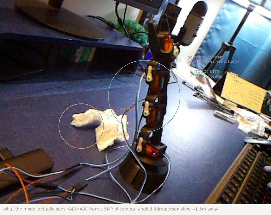
been tinkering with robot learning policies in simulation for a while now and wanted to make things work on a real robot setup. found a 3D printed 5 DOF robot off a youtube video which felt easy enough to build and work with as it literally just had SG90 servo motors as actuators making my experiment pretty cheap. i wanted to know what the bare minimum is for a robot arm to learn to reach and pick things up. no pretrained VLM backbone, no hardware encoders, no torque sensors, just SG90s and a pi camera.

with the cheap open loop servos, a stiff plastic arm, pixelated noisy images and only 50 teleoperated demos i wasn’t honestly thinking i would be able to get it to work at all but to my surprise, i could see the robot come to life and pick up the tissue it was trained on with a ~23% success rate

i have put all the instructions on assembly, teleop, model training along with the code for each in this github repository. it also contains the link to the hugging face checkpoint i uploaded. feel free to use it, fork it or contribute to it

stripping it down to bare minimum

before this, i did an experiment with an old VLA called Octo which i used to train a simulated Franka Panda arm where i was testing positive transfer of pretrained information. i finetuned with 100 episodes and got success in a reach task. it worked but i couldn’t really tell how much was pretrained knowledge, how much was actually my data which led to the task success, or how much was it the precise inverse kinematics and PID controllers in the Franka arm which led to success. too many things were doing the work for me. so this time, no VLM backbone (we did use a resnet pretrained on ImageNet for image understanding, but no pretrained robot knowledge), no encoders which tell where the servo is currently positioned/rotated, we had to rely on the accuracy of the pulse width we sent and the servo reading that instruction properly. no torque sensors and a 3D printed plastic robot arm which i had to use a knife to carve out holes big enough to fit the servos properly.

why ACT?

i had a rough idea for an architecture, a pretrained CNN for image tokens, a transformer to encode joint actions, fuse them together and predict angles. before i could test that intuition claude suggested i look at ACT which was an existing behavior cloning policy. went through lerobot’s documentation on it and it fit what i needed, small model, works with few demos, and the architecture wasn’t far from what i was thinking anyway.

went through the ACT paper, realised how good of a setup these researchers had with their ALOHA, clutter free desk, leader follower arms etc. took the core algorithm and derived an implmentation for my hardware

interesting ideas this paper introduced

action chunking: predicting one step, executing, observing and predicting again naturally compounds more error. predicting multiple steps at once first eliminates the jerkiness of inference but also takes care of error compounding as the model learns trajectories and not iterative poses. even if a few steps are slightly off, the trajectory self-corrects. i understood it as giving someone instructions at turns to navigate vs showing the entire route on a map

conditional variational autoencoder: if we just directly use a transformer encoder without a CVAE we would be facing an issue where despite the target being achieved, an approach from the left and an approach from the right get averaged out and the arm tries to step in empty space as there is no encoded representation of specifically the style or direction of approach that was taken to reach target. we try to bake in this information through this layer.

a vanilla autoencoder would encode input into a compressed state z and then have another layer to decode it back to X’. a variational autoencoder goes further where instead of encoding to a fixed point in latent space it encodes to a distribution (mean and variance). this works really well for image generation because the latent space z when sampled as a distribution can output new values leading to new images getting created during decoding.

a conditional autoencoder means that we will now provide some context along with the input to the variational autoencoder. in our case the input is 50 action chunks, the context(conditional) is the current joint angles (observation), and the output of this CVAE will be a 32 dimension latent space called z. this z allows us to differnetiate a “left-approach” from a “right-approach”

there are other ways to handle variablity of approach paths. models like RT-2 predict actions one token at a time, they don’t predict trajectories so mode averaging doesn’t become an issue. diffusion action heads in policies like Octo have iterative denoising which prevents style/trajectory production at one shot. you could also just collect consistent demos at scale with the same strategy so there’s nothing to average over. mode averaging would hit the hardest in a small model where the entire action chunk has to be produced in one shot non-autoregressively, which is exactly our case

the architecture

the ACT policy is four modules stitched together. a vision backbone, a CVAE encoder, an observation fuser, and an action decoder.

class ACTPolicy(nn.Module):
    def forward(self, image, state, actions=None):
        """
        image: [B, 3, 480, 640]
        state: [B, 5] (normalized)
        actions: [B, chunk_size, 5] (normalized, training only)
        Returns: pred_actions [B, chunk_size, 5], mu, logvar
        """
        # Part B: Vision
        visual_tokens = self.vision(image)  # [B, 300, d_model]

        # Part A: CVAE (training) or zero latent (inference)
        if actions is not None and self.training:
            mu, logvar, z = self.cvae(state, actions)
        else:
            B = image.shape[0]
            z = torch.zeros(B, self.latent_dim, device=image.device)
            mu, logvar = None, None

        # Part C: Observation Fuser
        fused = self.fuser(visual_tokens, state, z)  # [B, 302, d_model]

        # Part D: Action Decoder
        pred_actions = self.decoder(fused)  # [B, chunk_size, 5]

        return pred_actions, mu, logvar

images gets converted into 300 visual tokens through the vision backbone. in parallel, CVAE compresses the action sequence into a style vector z. the fuser lets all of this multimodal information self-attend to each other, and the decoder cross attends action queries to fuser output to predict the next 50 joint angles (we will talk about this in detail later)

the image encoder:
we use resnet18 as the vision backbone to get a general understanding of images

class VisionBackbone(nn.Module):
    """ResNet18 → 300 visual tokens with positional embeddings."""

    def __init__(self, d_model=256):
        super().__init__()
        resnet = torchvision.models.resnet18(
            weights=torchvision.models.ResNet18_Weights.IMAGENET1K_V1
        )
        # Keep everything except avgpool and fc
        self.backbone = nn.Sequential(*list(resnet.children())[:-2])
        # Project 512 channels → d_model
        self.proj = nn.Conv2d(512, d_model, kernel_size=1)
        # 2D positional embeddings for 15x20 grid (480/32=15, 640/32=20)
        self.register_buffer(
            "pos_embed", sinusoidal_2d_pos_embedding(15, 20, d_model)
        )

    def forward(self, image):
        """image: [B, 3, 480, 640] → [B, 300, d_model]"""
        features = self.backbone(image)  # [B, 512, 15, 20]
        features = self.proj(features)   # [B, d_model, 15, 20]
        tokens = features.flatten(2).permute(0, 2, 1)  # [B, 300, d_model]
        tokens = tokens + self.pos_embed  # add positional encoding
        return tokens

not going into the internals of the network but it basically is an 18 layer CNN pretrained on ImageNet which was itself an image encoder trained on 1.2M images in 1000 categories so it knows about edges, textures, shapes and objects. it also has skip connections in between layers to avoid vanishing gradients (something i’ve talked about in my LLM blog post. the last two layers of resnet, avgpool and fc are more used for classification tasks where they do collapse the pixel grid into a 1x1 layer and then map the 512-dim representation to 1000 dimensions which are the 1000 classifications of ImageNet. as we only care about the spatial map, we remove these layers from the vision layer

through the CNN we downsample the 480x640x3 image into 15x20x512 (a 32x downsampling). this then goes through another convolutional layer reducing dimensionality from 512 -> 256. we then add a sinusoidal positional embedding and flatten the matrix out to output 300 image tokens, 256 dimensions each.

conditional variational autoencoder:
i already covered what the CVAE does and why we need it above. here is the implementation for the same

class CVAEEncoder(nn.Module):
    """Compresses (state, action_sequence) into latent z. Training only."""

    def __init__(self, d_model=256, latent_dim=32, chunk_size=50, state_dim=5, n_layers=4):
        super().__init__()
        self.cls_token = nn.Parameter(torch.randn(1, 1, d_model) * 0.02)
        self.state_proj = nn.Linear(state_dim, d_model)
        self.action_proj = nn.Linear(state_dim, d_model)
        self.pos_embed = nn.Embedding(1 + 1 + chunk_size, d_model)  # CLS + state + actions

        encoder_layer = nn.TransformerEncoderLayer(
            d_model=d_model, nhead=8, dim_feedforward=d_model * 4,
            dropout=0.1, activation="relu", batch_first=True,
        )
        self.transformer = nn.TransformerEncoder(encoder_layer, num_layers=n_layers)
        self.mu_proj = nn.Linear(d_model, latent_dim)
        self.logvar_proj = nn.Linear(d_model, latent_dim)

    def forward(self, state, actions):
        """
        state: [B, 5], actions: [B, chunk_size, 5]
        Returns: mu [B, latent_dim], logvar [B, latent_dim], z [B, latent_dim]
        """
        B = state.shape[0]
        cls = self.cls_token.expand(B, 1, -1)                    # [B, 1, d]
        state_token = self.state_proj(state).unsqueeze(1)         # [B, 1, d]
        action_tokens = self.action_proj(actions)                 # [B, chunk, d]
        sequence = torch.cat([cls, state_token, action_tokens], dim=1)  # [B, 2+chunk, d]

        # Add positional embeddings
        pos_ids = torch.arange(sequence.shape[1], device=sequence.device)
        sequence = sequence + self.pos_embed(pos_ids)

        encoded = self.transformer(sequence)  # [B, 2+chunk, d]
        cls_out = encoded[:, 0]               # [B, d]

        mu = self.mu_proj(cls_out)            # [B, latent_dim]
        logvar = self.logvar_proj(cls_out)    # [B, latent_dim]

        # Reparameterization trick
        std = torch.exp(0.5 * logvar)
        eps = torch.randn_like(std)
        z = mu + std * eps

        return mu, logvar, z

the state_token, which is just current joint angles, acts as the conditional context which goes in both in the CVAE and in the action decoder later. we could have added the image to the context as well but we only wanted CVAE to train on the style/approach of the trajectory and not where the object is or how it looks. this trimming also helped us keep the latent space small (32 dim)

the state_token gets projected from the 5 joint angle dimensions to 256 dimensions. same happens to the next 50 chunks of actions extracted from training data. we concatenate the CLS token, current state and future 50 action tokens together, add positional embeddings, and then pass it through the encoder transformer.

the CLS token actually gets trined to attend to all the action tokens. we then take the output CLS token [B, 1, 256] and project it down to the latent space of 32 dimensions, splitting it into mean and log variance. these parameterise a gaussian distribution in the style space. log(var) because we want to allow negative values as well. the point of outputting a distribution instead of a single fixed vector is that we get a region to sample from, which is what gives us variability across different trajectories

the only problem though is that we can’t differentiate the dsitribution w.r.t the mean or standard deviation as we don’t really have a functional relation between them

\[z \sim \mathcal{N}(\mu, \sigma^2) \implies \frac{\partial z}{\partial \mu} = \text{undefined (random)}\]

but if we add some noise, the equation becomes z = f(mu,sigma) which is easy to backpropogate through. this is called reparameterization:

\[z = \mu + \sigma \cdot \epsilon, \quad \epsilon \sim \mathcal{N}(0, 1)\]

now gradients flow cleanly through $\mu$ and $\sigma$ because $\epsilon$ is just a constant with respect to the model parameters:

\[\frac{\partial z}{\partial \mu} = 1, \quad \frac{\partial z}{\partial \sigma} = \epsilon\]

mathematically the same distribution, but the computation graph is differentiable.

observation fuser:
is a self attention encoder-only transformer like BERT. this is used to fuse everything into the same latent space. the image tokens, the z token having the trajectory style learning, and the current joint angles we call state (5 dimensions currently)

class ObservationFuser(nn.Module):
    """Fuses visual tokens + state + z into enriched representations."""

    def __init__(self, d_model=256, latent_dim=32, state_dim=5, n_layers=4):
        super().__init__()
        self.state_proj = nn.Linear(state_dim, d_model)
        self.z_proj = nn.Linear(latent_dim, d_model)

        encoder_layer = nn.TransformerEncoderLayer(
            d_model=d_model, nhead=8, dim_feedforward=d_model * 4,
            dropout=0.1, activation="relu", batch_first=True,
        )
        self.transformer = nn.TransformerEncoder(encoder_layer, num_layers=n_layers)

    def forward(self, visual_tokens, state, z):
        """
        visual_tokens: [B, 300, d], state: [B, 5], z: [B, latent_dim]
        Returns: [B, 302, d]
        """
        state_token = self.state_proj(state).unsqueeze(1)  # [B, 1, d]
        z_token = self.z_proj(z).unsqueeze(1)              # [B, 1, d]
        fused = torch.cat([visual_tokens, state_token, z_token], dim=1)  # [B, 302, d]
        return self.transformer(fused)

we project the state and z vector to match the model dimensions and concatenate them with visual tokens. all of them go through 4 layers of self attention and feedforward networks post which they get a mutual understanding of approach, space, and state

action decoder: this layer decodes the fuser output [B,302,d] into the next 50 chunks of actions. given a state(including the image and joint angles), it takes information from this space on what the future joint angles shoud look like

class ActionDecoder(nn.Module):
    """Cross-attends learned queries to fuser output → predicts action chunk."""

    def __init__(self, d_model=256, chunk_size=50, state_dim=5, n_layers=1):
        super().__init__()
        self.query_embed = nn.Embedding(chunk_size, d_model)

        decoder_layer = nn.TransformerDecoderLayer(
            d_model=d_model, nhead=8, dim_feedforward=d_model * 4,
            dropout=0.1, activation="relu", batch_first=True,
        )
        self.transformer = nn.TransformerDecoder(decoder_layer, num_layers=n_layers)
        self.action_head = nn.Linear(d_model, state_dim)

    def forward(self, fuser_output):
        """fuser_output: [B, 302, d] → [B, chunk_size, state_dim]"""
        B = fuser_output.shape[0]
        queries = self.query_embed.weight.unsqueeze(0).expand(B, -1, -1)  # [B, chunk, d]
        decoded = self.transformer(tgt=queries, memory=fuser_output)       # [B, chunk, d]
        return self.action_head(decoded)  # [B, chunk, state_dim]

the transformer decoder has both self and cross attention. the learned queries here are 50 trainable vectors [50, 256] which figure out how the action should be at step 0, step 1…step 49. each query gets trained to predict the state/action of that query index. they start random and learn through training to ask the right question to the fuser output. for example query 0 would specialise to ask what happens right now given the image, current state and the style? query 49 might specialise in what happens 8 seconds later (depends on frame rate/frequency). i think of it as learned semantic meaning about the temporal role of each step of the chunk.

how cross attention works: each query does a dot product with keys from the fuser output. think of the fuser output creating K and V after which we apply the same attention formula QK^T). the eventual value vector with which we do a weighted sum also comes from the fuser output. so each query’s output is a mix of the fuser tokens it attended to the most. imagine the gripper has picked up the tissue and wants to retract now. this understanding of retracting comes from the later stages of the query embedding attending to the combination of the state and image knowledge

before cross attention the 50 queries also attend to each other because we want these queries to know what is happening. note that we don’t attach a causal attention mask to the attention layers as we want the queries to know future states as well for temporal coherence. regarding the layering of the decoder transformer, we don’t need more than 1 layer as most of the reasoning has been done by the fusion layer. ACT paper also suggests 1 for simple tasks and maybe more for more DOF, more complicated manipulation like bimanual

what did the cross attention layer actually learn?

i wanted to see if the model actually learned anything semantically meaningful from the 50 demos or was it just memorizing trajectories?

hooked into the cross attention weights of decoder and visualized what each of the 50 queries looks at when making predictions

the queries specialize temporally. the query embeddings learned to attent to temporal steps on their own. query 0 learned to attend more to the early steps without explicitly asking it to do so. at step 50 (arm is mid-descent), query 0 focuses attention tightly on the arm’s current position in the image. query 25 shifts attention down to where the tissue is sitting on the workspace. query 49 spreads attention broadly across the lower frame, planning the retraction. each query learned to ask a different question about the scene depending on how far into the future it’s predicting. was pretty cool to see

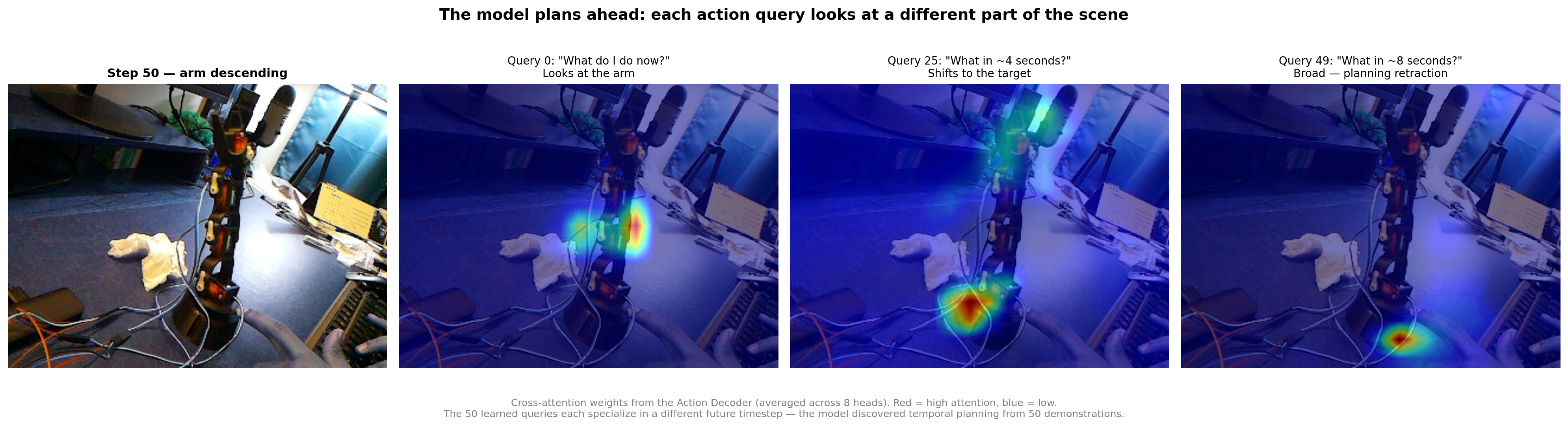
attention follows the arm dynamically. if i look at just query 0 (the immediate next action) across different points in the episode, the attention hotspot physically moves with the arm. at step 0 it’s focused on the upper-center of the image where the arm sits at home. by step 50 the hotspot has moved to mid frame as the arm descends. at step 100 it’s in the lower frame near the tissue. the model wasnt memorizing a fixed attention pattern, it was dynamically tracking the arm in real time based on what the camera saw.

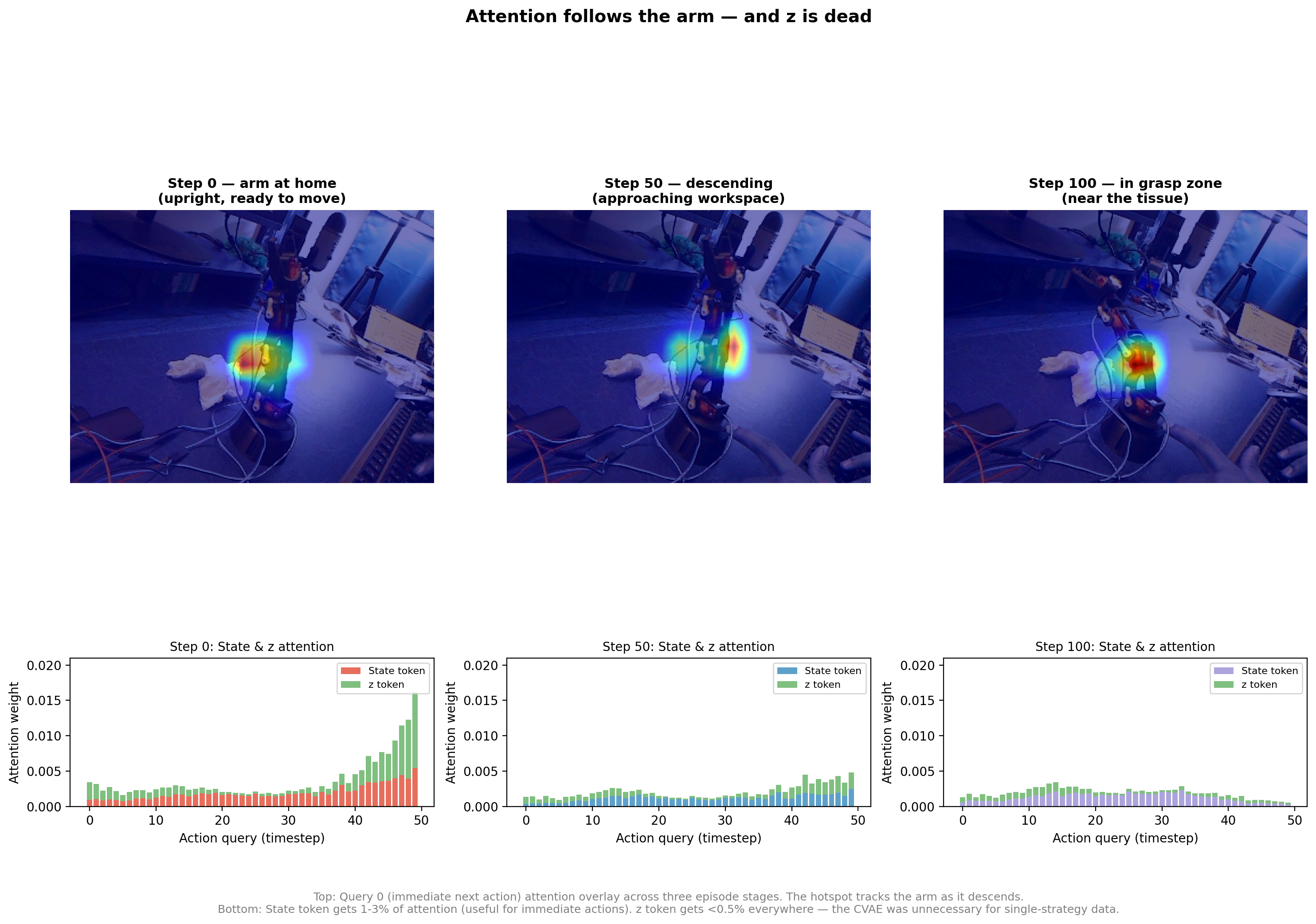
z gets ignored. the bottom row of that second image shows the z token getting less than 0.5% of attention from all queries across all timesteps. the model wasn’t using it at all. itm ade ense because our data collection didn’t have a lot of variety in ways to approach and reach a target. the KL loss also pushed it toward carrying zero information (have shared the training loss numbers below)

training

the loss function. there are two components of loss, L1 reconstruction loss on the predicted joint angles, and KL divergence to regularize the CVAE:

def compute_loss(pred_actions, target_actions, pad_mask, mu, logvar, beta=10.0):
    """L1 reconstruction + KL divergence."""
    # L1 loss, masked for padded positions
    l1 = F.l1_loss(pred_actions, target_actions, reduction="none")  # [B, chunk, 5]
    mask = (~pad_mask).unsqueeze(-1).float()  # [B, chunk, 1]
    l1 = (l1 * mask).sum() / mask.sum() / STATE_DIM

    # KL divergence: push q(z|x) toward N(0,1)
    kl = -0.5 * torch.mean(1 + logvar - mu.pow(2) - logvar.exp())

    loss = l1 + beta * kl
    return loss, l1.item(), kl.item()

the L1 loss is just the mean absolute error between predicted and actual joint angles for each of the 50 future steps. the pad_mask handles episode boundaries, if an episode has 100 steps and we’re at step 80, the chunk needs 50 future actions but only 20 are real. the remaining 30 get padded with the last state and masked out so the model isn’t penalized for predicting beyond the episode end.

the KL term pushes the CVAE’s learned distribution toward standard normal. beta=10 weights KL heavily so z doesn’t try to encode noise

loss trajectory. trained on a rented RTX 4080S on vast.ai ($0.08/hr). 100K steps took 3 hours

for the L1 loss, we could see how the first 100 steps were random predictions where the model was slowly learning rough angle ranges. at the 2-15k training step, it could understand genreal trajectory and was finetuning movements. from 50-100K the model worked on polishing the predictions, the improvements were slow but consistent

the KL trajectory had to be visualised on the log scale because it collapsed from 0.249 to 0.000001, the CVAE learned to encode literally nothing into z. this is the same conclusion we saw in the attention visualization: the model ignores z because z carries no information. all 50 demos approach from roughly the same angle, so there’s no style to capture. for the ACT paper’s bimanual tasks with genuine approach variation this would look different

all in all, the model had learned the behavior from $15 worth of hardware, $0.25 of compute and 25 minutes of demos. now we had to deploy this on the physical arm

distributed inference between raspi and mac over tcp

the pi handled the camera and motors, mac handled the model inference(brain). needed a fast communication between the two devices so made them talk over a TCP socket on local network

why tcp and not http. a REST API would mean a new HTTP request every cycle, connection negotiation, headers, content type, etc. when yo’re working with real time system, every ms counts so couldn’t afford the overhead. we anyway had a slow control loop(5Hz) bottlenecked by the mac inference performance. we sent one JPEG and got back 5 floats, 5 times a second

the protocol. 4-byte big-endian length prefix followed by JSON. dead simple:

def send_msg(sock, data):
    """Send a length-prefixed JSON message."""
    raw = json.dumps(data).encode()
    sock.sendall(struct.pack(">I", len(raw)) + raw)

def recv_msg(sock):
    """Receive a length-prefixed JSON message."""
    raw_len = recv_exact(sock, 4)
    msg_len = struct.unpack(">I", raw_len)[0]
    raw = recv_exact(sock, msg_len)
    return json.loads(raw.decode())

the receiver reads exactly 4 bytes, unpacks the message length and reads exactly that many bytes. no delimiter scanning, no chunked transfer encoding, no parsing ambiguity. for the image frames, the pi sends a JSON header containing the joint state + jpeg_size, then dumps the raw JPEG bytes right after. the mac knows exactly how many bytes to read because the header told it. no base64 encoding waste

where the time goes. the round trip involves pi camera capturing and encoding JPEG taking ~50ms. sending the ~30-50KB JPEG over wifi to the mac takes ~40ms. model inference on MPS (18.7M params, one forward pass through resnet + fuser + decoder) takes ~100ms(slow). sending the 5 action values back and executing them on the servos took another 20ms leading to a ~200-250ms latency (5FPS/Hz)

now the training data was collected at 6Hz so there was a 1Hz gap which meant that the arm would move slightly more between inference steps than the model was trained on. luckily for a coarse reach and pick task this didn’t hurt us but this is dfinitely a production system red flag if you’re wokring on super precise manipulation tasks

temporal ensembling

this was a new concept for me so felt like writing about it

as mentioned in the paper, during inference, we could average out the next step by looking at the specific step in all the previous action chuncks that got generated and averaging them

what this means is at every inference step, the model predicts 50 future actions (the full chunk). at the next step, it predicts another 50 future actions. these chunks overlap. step 5 appears in the predictions of every chunk started from steps 1 through 5. so for step 5 we have 5 separate predictions. instead of using just the step 5 that got generated latest, we average out these values(adding a weighted importance to how long ago that step 5 was generated)

the chunk started at step 1 predicted actions for steps 1-50. step 5 is at index 4 of that chunk. the chunk started at step 2 predicted steps 2-51. step 5 is at index 3. the chunk started at step 5 predicted steps 5-54. step 5 is at index 0. each of these predictions comes from a different observation (different camera frame, different joint state) so they’re not identical but they should be close.

temporal ensembling takes the weighted average of all these overlapping predictions. the weight is exponential decay based on the index within the chunk: w = exp(-0.01 * i). predictions from index 0 (the freshest chunk, just predicted) get weight 1.0. predictions from earlier chunks (higher index) get slightly less weight.

with decay=0.01 the falloff is gentle, all recent predictions contribute roughly equally. the effect is a smoothing filter on the predicted trajectory. if one chunk had a slightly off prediction (maybe the camera caught a weird frame), the other 4 chunks dilute it. this works great for continuous joint angles.

i should have removed ensembling from the gripper though
the gripper is binary: open (1.0) or closed (0.0). when the model decides “close now,” only the most recent chunk’s prediction says 0.0. the 4 older chunks still predict 1.0 (they were made from earlier observations when the gripper should have been open). the weighted average produces something like 0.8, then 0.6, then 0.4, then finally 0.0 over several steps. the gripper fades closed instead of snapping.

at 5Hz, 3-4 steps of gripper lag means 600-800ms. the arm arrives at the tissue, the model says close the gripper, but the ensembled signal is still “mostly open.” by the time the gripper actually closes, the arm has already started retracting. the gripper closes on empty air above where the tissue was.

for binary/categorical actions (0 for open, 1 for close) I’m not sure if temporal ensembling was the best thing to do

we got a 23% success rate!

when i replayed training episodes through the model and compared predictions to actual recorded actions, mean joint error was just 0.68° across all joints. the servos themselves have 2-3° of physical slop anyway so the model was more precise than the hardware. gripper accuracy was 99.6%, which meant almost perfect classification of open vs closed.

as this was already existing training data, it felt like the model fit really tightly to these exmaples. when I deployed it on the robot and captured new frames and state, I got 7/30 tests passing.

position	success	rate
center	4/10	40%
left	2/10	20%
right	1/10	10%
total	7/30	23%

10 trials per position, tissue placed consistently within each zone. success = tissue lifted off table and held for 2+ seconds

what went wrong

the gripper timing from temporal ensembling was the biggest factor. the arm would reach the tissue correctly, the wrist would tilt down, everything looked right and then the gripper would close 600ms late. in several trials the arm arrived at the tissue, hovered for a moment with the gripper fading from open to closed, and by the time it actually gripped the retraction trajectory was already pulling the arm back up. it closed on air.

the position bias in training data was the second factor. most of my 50 demos had the tissue near center of the workspace. left and right placements were effectively out-of-distribution. the success rate gradient (40% center → 20% left → 10% right) directly mirrors how many training demos the model saw for each region. this isn’t a model problem, it’s a data diversity problem.

servo torque at the grasp point was the third factor. the SG90 has 1.8 kg·cm of torque. at full arm extension the lever arm means the shoulder servo is fighting the weight of the entire arm plus the tissue. in some trials the arm visibly sagged 1-2cm at the grasp point, shifting the gripper off target just enough to miss. sometimes it also started vibrating aggresively not able to carry more load

what actually worked though

the trajectory shape was understood well by the model. every action from reaching forward, wrist tilting down, approaching the workspace, attempting to grip and retracting upward was a learned capability. the motion looked like a robot that knew what it was doing. the timing of the approach phase was also consistent and the wrist tilt angle matched what i demonstrated. when it did succeed it looked confident

most of the failures were about precisions and not understanding the task

what would improve this

the biggest thing is data. most of my 50 demos had the tissue in the center because that’s where i kept placing it without thinking, and the 40% center vs 10% right gap is the model telling me exactly that. more diverse tissue positions, more episodes (100+), and maybe a leader-follower teleop setup instead of keyboard so the demos themselves are smoother. i think volume and diversity of data alone would bump the accuracy up significantly

the second thing is spatial understanding. one angled camera at 640x480 from ~1m away gives maybe 10 pixels of useful signal on the gripper fingers. a wrist camera would give millimeter-level feedback right at the contact point, and the ACT paper used 4 cameras for the same reason. better spatial input would make the grasp much more reliable

this was a good experiment. the pipeline proved that behavior cloning works even on the leanest setup, $15 of hardware, one noisy camera, 50 demos, plastic servos with no feedback. ACT is a really good fit for this kind of thing, simple low-DOF tasks on cheap hardware with small datasets. the architecture is small enough to train in under 3 hours for $0.02 and run inference at 5Hz on a laptop. for anything more complicated like bimanual manipulation or tasks that need precision you’d want better hardware and more data, but for getting a robot to learn a behavior from scratch this worked way better than i expected!