what transfers when nothing matches
tech ·finetuning a cross-embodied VLA on synthetic renders, different actions, and zero teleoperation
the setup
i was exploring vision language action models as part of a broader dive into embodied AI. i already trained an RL policy (SAC) that could reach targets with a simulated franka panda arm in MuJoCo. got a 100% success rate with a small MLP (2 hidden layers, batch size 256) feeding it joint positions, velocities, fingertip coordinates and target coordinates as a 20 dim vector, outputting joint angle deltas. since i eventually want to train an actual robot, i wanted to explore a more realistic setup, feeding camera images felt like a more realistic setup instead of a simulation state vector that doesn’t exist in the real world.
i picked octo, a 93M parameter VLA pretrained on 800K filtered high quality demonstrations from the open x-embodiment dataset. there were other options as well. RT-1-X is smaller (35M params) but the action format is baked into the output layer, so adapting it to a new action space means changing the entire output scheme (a lot of training). RT-2-X and openVLA are billions of parameters, too slow to tinker with. octo hit a sweet spot where it is small enough to iterate fast and architecturally designed for fine-tuning. and the action head is replaceable, swapping to a new robot’s action space is just replacing the head and fine-tuning on a few hundred demos while the backbone handles the rest.
what i didn’t expect is how far outside the intended use case i’d end up pushing it. my setup had three things that were simultaneously out of distribution: cartoonish MuJoCo renders instead of real camera images, joint angle deltas instead of end-effector actions (i replaced the entire pre-trained action head), and demonstrations from an RL policy instead of a human teleoperator. none of this is what I think octo was designed for. and it still worked. 90% success, finetuned on 300 demos and 25K gradient steps (batch of 16 steps per gradient descent), ~47 minutes on a rented GPU.
tinkering through the failures and eventually getting there gave me some concrete thoughts on what actually transfers in these foundation models and what doesn’t. this experiment was a part of my speedrunning robotics sprint which I’ve written about here. this is the code repository which you can use to reproduce this experiment. the model checkpoints are uploaded here
the rl teacher
before getting to octo, quick context on the policy that generated the training data. SAC (soft actor-critic) is an off-policy RL algorithm where two neural networks learn together: the actor picks actions given the current state, the critic evaluates how good a (state, action) pair is. the policy sees 20 floats: 7 joint angles, 7 joint velocities, 3 fingertip xyz coordinates, 3 target xyz coordinates and outputs 7 normalized joint angle deltas in [-1, 1], scaled by 0.1 radians per step (we scaled the output down because we wanted to keep movements small and smooth).
the reward function is a simple euclidian distance between the fingertip and the target:
def step(self, action):
    action = np.clip(action, -1.0, 1.0)
    delta = action * ACTION_SCALE          # 0.1 rad per unit
    new_qpos = self._current_qpos + delta

    obs_dict = self._env.step(new_qpos)
    self._current_qpos = obs_dict["joint_pos"].copy()
    self._step_count += 1

    dist = obs_dict["dist"]
    reward = -dist                          # closer = better

    terminated = bool(dist < SUCCESS_DIST)  # 5cm threshold
    truncated = bool(self._step_count >= MAX_STEPS)

    if terminated:
        reward += 1.0                       # bonus on success

    return self._flatten_obs(obs_dict), reward, terminated, truncated, info
negative distance each step, +1 bonus when the fingertip gets within 5cm of the target. that’s it. no shaping, no curriculum. kept it lean
this took 5 failed training runs before it worked. the failures weren’t about hyperparameters, they were about the task itself. i had targets placed at z=0.33m (table surface), but only 0.49% of random joint configurations could physically reach that zone. the arm couldn’t stumble into success often enough for RL to bootstrap from. raising the target zone to z=[0.40, 0.75] bumped reachability to 2.9%, and the same SAC config that was stuck for 4 runs hit 100% success on run 5. 300K environment steps and 20/20 evaluation episodes with ~95 steps average to reach. the policy needs a decent enough probability of success to actually work (maybe if I trained it on enough steps, it could reach the 0.49% environment as well)
this policy becomes the teacher. its job now was to generate demonstrations for octo. the question is whether a foundation model can learn the same task from those demonstrations using only camera images, a replaced action head, and zero reward signal. and if it can, what part of the pretraining is actually doing the work?
what is octo
to understand what might transfer and what won’t, we will do a short deep dive into how octo is structured because the architecture was explicitly designed to separate the transferable parts from the disposable ones.
a vision language action model takes camera images and a language instruction and directly outputs motor commands. no separate perception pipeline, no planning module, no inverse kinematics. pixels in, actions out, all through a single model
octo is a multi-uni collaborative effort between academics from UC Berkeley and Stanford. it was pre-trained on 800K real robot trajectories from the open x-embodiment dataset, demonstrations from 22 different robot embodiments doing tabletop manipulation tasks with real cameras. the hypothesis was that if you train on enough visual and morphological diversity, the backbone learns general spatial reasoning that transfers to new robots and if you design the architecture right, adapting to a new robot should be as simple as swapping the action head and fine-tuning on a few hundred demos (thats exactly what we will be doing)
the architecture has three stages: tokenize the inputs, process them through a transformer, decode actions with a diffusion head
tokenization:
language and image tokens are generated separately. language goes through T5-Base, a frozen 111M parameter text encoder. “reach the green target” becomes ~16 tokens of 768 dimensions each. T5 is never updated during octo’s training or fine-tuning, it is just used to generate tokens out of the action command/text. we do get the added benefit of contextual knowledge from the pretrained T5 transformer, which gets added to the token’s embeddings
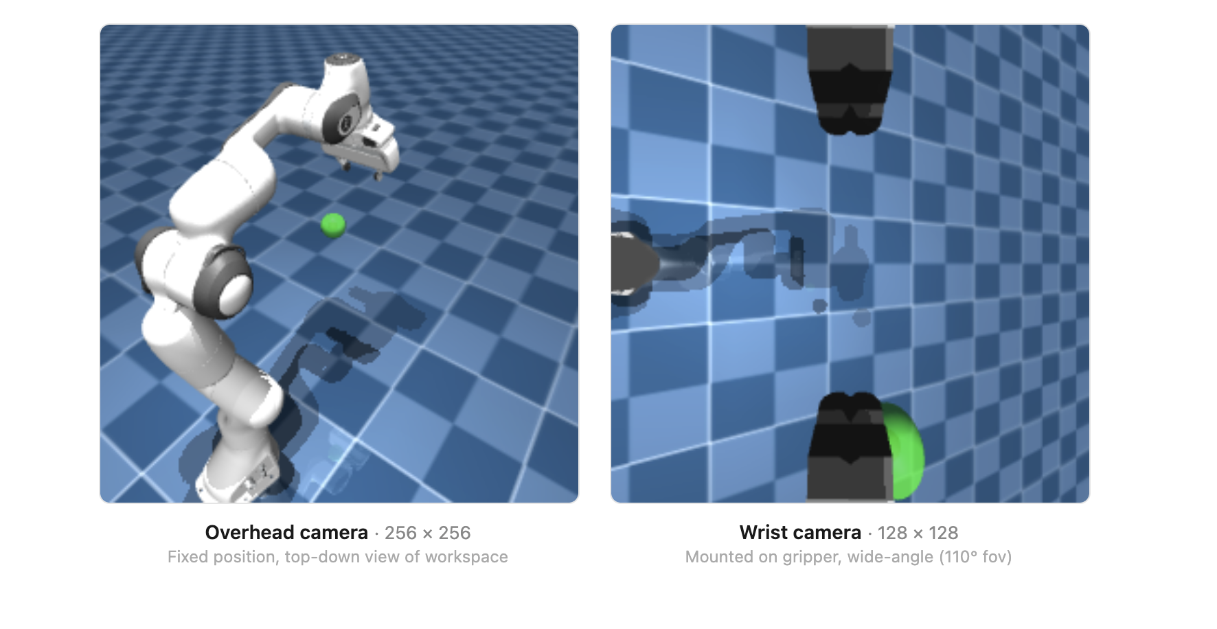
images go through a deliberately shallow CNN with just 2-3 convolutional layers. a 256x256 overhead camera image becomes 256 tokens (16x16 patch grid), each 384 dimensions. a 128x128 wrist camera image becomes 64 tokens (8x8 grid). most vision models do the opposite where they have deep CNNs (RT-1 uses an 18-layer EfficientNet) with a small transformer on top. octo inverts this: minimal CNN, big transformer. the idea is that with 800K trajectories, the transformer can learn visual features from raw patches on its own and unlike a CNN, its attention mechanism can directly cross-reference image patches with language tokens, so “green target” in the instruction gets grounded to the actual green pixels in the scene.
each token also gets position embeddings that encode both where it sits spatially and what type of input it is (language token vs overhead image token vs wrist camera token vs which time step). this is how the transformer knows what it’s looking at.
transformer backbone:
12 layers, 12 attention heads, 768 dimensions per token (every token flowing through the transformer is a vector of 768 floats). the same Q/K/V self-attention as GPT-2 arch. queries, keys, values, dot-product attention, feedforward layers, residual connections, layer norm. if this is all jargon to you i’ve done a deep dive on building a transformer from scratch here
the difference is the attention mask. GPT-2 uses a simple triangular causal mask (each token sees everything before it). octo uses a block-wise mask:

language tokens only attend to other language tokens, the instruction is processed in isolation. image tokens attend causally across time, the current frame can see the previous frame but not vice versa. and then there’s the readout token (which kinda eventually summarises the connections between all tokens)
the readout token is the key design decision. it can see everything including language, images, history of what all happened during training. it builds a complete summary of the visual situation without influencing how the backbone processes images and language as it can’t be read by other tokens.
this is important because anything attached to the readout token (action heads) can be swapped, removed, or replaced without changing the backbone’s learned representations at all. the backbone processes images and language exactly the same way regardless of what action head is plugged in. this is what makes the action head replaceable and is the architectural feature i ended up relying on most heavily.

diffusion action head:
the readout embedding (768 floats) summarizes the full visual context. now we need to turn that into motor commands. octo uses a diffusion head which is a small MLP (3-4 linear layers, ~2-5M parameters) that generates actions by iterative denoising.
during training: take a real action from a demonstration, add random noise at a random level, and train the MLP to predict what noise was added. the MLP sees the noisy action, the readout embedding (visual context), and the noise level.
during inference: start from pure random noise and run the MLP 20 times. each pass predicts and subtracts a layer of noise. after 20 steps, you have a clean action. the transformer runs once to produce the readout embedding, then only the small diffusion head iterates so it stays fast.

we could have trained the mlp to directly predict the action by going with an MSE loss, but MSE can only output one action which means that if reaching from the left and reaching from the right are both valid, MSE averages them and you get an action that goes straight into the table. diffusion naturally handles the situation where there are multiple paths to success. different random starting noise flows toward different valid actions during denoising.
the head outputs an action chunk of 4 consecutive actions (7 dimensions each = 28 floats). one transformer forward pass produces 4 control steps. this is faster than running the full model every step, this also ensures smoothness as we get 4 smooth transitions in one pass (less jerky)
from rl policy to training data
so we have a backbone that supposedly transfers and an action head we’re throwing away. now i need training data and this is where the domain gaps really start stacking up. the SAC policy lives in state vector land, but octo needs camera images. to create demonstrations, i needed to capture what the cameras sees alongside what the policy does.
added two cameras to the MuJoCo scene. one was an overhead camera at a fixed position looking down at the workspace (256x256), and the other was a wrist camera mounted on the gripper body looking forward downward (128x128). the target is a semi-transparent green sphere with no physics collision
for ep in range(N_EPISODES):
    obs = env.reset()

    for step in range(200):
        # render both cameras from the same MuJoCo state
        overhead_img = overhead_renderer.render(mujoco_env.data)
        wrist_img = wrist_renderer.render(mujoco_env.data)

        # policy picks action
        # non-deterministic for trajectory diversity adds Gaussian noise so same target gets different approach paths
        action, _ = policy.predict(obs, deterministic=False)

        # record the actual joint delta
        raw_action = np.clip(action[0], -1.0, 1.0)
        joint_delta = raw_action * ACTION_SCALE

        all_overhead_images.append(overhead_img)
        all_wrist_images.append(wrist_img)
        all_actions.append(joint_delta.astype(np.float32))

        obs, reward, done, info = env.step(action)
        if done[0]:
            break

    episode_starts.append(len(all_overhead_images))
the critical detail is deterministic=False. SAC’s actor outputs a mean and standard deviation. deterministic mode takes the mean where as non-deterministic samples from the distribution. this means the same target position produces different approach trajectories each time allowing for a vareiety of paths to be fed to training. this diversity turns out to be the single most important factor in the entire fine-tuning pipeline. will talk about it later.
we collect 300 episodes, ~30K total frames saved as flat numpy arrays including overhead images, wrist images, actions, and episode boundary indices
what we changed in octo
this is where we deliberately break the things that aren’t supposed to transfer, and keep the things that are. we keep the language encoder, the image tokenizer and the transformer backbone as it is while replacing the action head. octo’s pre-trained head outputs end-effector deltas: (dx, dy, dz, rotations, gripper). our task needs 7 joint angle deltas. same dimensionality (7) by coincidence, but completely different physical meaning. our new diffusion head is initialized with random weights. all 800K demonstrations worth of “how to move a gripper through space” are gone from the action head. the backbone’s spatial reasoning is all that carries over.
# replace the action head completely
config["model"]["heads"]["action"] = ModuleSpec.create(
    DiffusionActionHead,
    action_horizon=ACTION_HORIZON,   # predict 4 future actions at once
    action_dim=ACTION_DIM,           # 7 joint deltas
    readout_key="readout_action"     # read from the same readout token
)

# build new model from modified config
model = OctoModel.from_config(
    config,
    pretrained_model.example_batch,
    pretrained_model.text_processor,
)

# copy pre-trained backbone weights into new model
# new action head stays random — nothing to copy
merged_params = merge_params(model.params, pretrained_model.params)
model = model.replace(params=merged_params)
merge_params is doing the important work here. it walks both parameter trees, copies every weight that exists in both (the 90M+ backbone and CNN params), and leaves the new action head’s random weights untouched. we keep the expensive pre-training and only need to learn the cheap head from scratch.
the loss function is a two-step forward pass. first the tokenizers and transformer backbone run to produce the readout embedding which is the 768-float vector summary of what the pipeline learns (“green target placed in front of robot arm currently fully at rest”) then the diffusion head takes that embedding and computes the noise prediction loss against the ground truth action from our demonstrations.
def loss_fn(params, batch, rng, train=True):
    bound_module = model.module.bind({"params": params}, rngs={"dropout": rng})

    # step 1: images → CNN → tokens, language → T5 → tokens, all → transformer → readout
    transformer_embeddings = bound_module.octo_transformer(
        batch["observation"],
        batch["task"],
        batch["observation"]["timestep_pad_mask"],
        train=train,
    )

    # step 2: readout → diffusion head → loss (add noise to real action, predict noise, MSE)
    action_loss, action_metrics = bound_module.heads["action"].loss(
        transformer_embeddings,
        batch["action"],
        batch["observation"]["timestep_pad_mask"],
        batch["action_pad_mask"],
        train=train,
    )
    return action_loss, action_metrics
if you’re used to PyTorch, model.module.bind(params) is the JAX/Flax equivalent of a model that already owns its parameters. in Flax, the architecture and weights are separate objects, where you “bind” them together before a forward pass. As a pytorch user, this was completely new syntax for me but claude code told me not to worry :D
the training step compiles down to a single JIT’d function(again a python annotation I had never used):
@jax.jit
def train_step(state, batch):
    rng, dropout_rng = jax.random.split(state.rng)

    # forward + backward in one call (PyTorch equivalent: loss.backward())
    (loss, info), grads = jax.value_and_grad(loss_fn, has_aux=True)(
        state.model.params, batch, dropout_rng, train=True
    )

    # apply gradients (PyTorch equivalent: optimizer.step())
    new_state = state.apply_gradients(grads=grads, rng=rng)
    return new_state, loss, info
training config: batch size 16, AdamW with linear warmup from 0 to 3e-4 over 100 steps then constant, T5 encoder frozen. 25K steps on a rented RTX 4080S via Vast.ai, ~47 minutes total. the first train_step call takes ~30 seconds while JAX compiles the computation graph, then every subsequent step is fast (i think that is the advantage over pytorch, will go over jax properly later)
what I learned
even with the right architecture and pre-trained weights, it took me a few hit, tries and failures to get the transfer working. some observations(failures) from my experiments
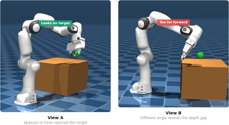
depth needs two eyes: the first run used a single overhead camera. 100 deterministic demos, 10K fine-tuning steps. loss dropped nicely from 1.42 to 0.60. during evaluation the arm would approach the target, get within 0.097m (almost the 0.05m success threshold), then drift away. every single episode. 0% success.
i realised that the problem was depth, the model didn’t get spatial understanding just using one camera angle. from one overhead viewpoint, the model couldn’t tell whether the gripper was in front or back of the target. they overlapped in the image. the arm would reach the right 2D position and then just oscillate on the third dimension with no signal to correct itself.
adding a wrist camera (128x128, mounted on the gripper) changed the information the model had access to. now the target sphere grows larger in the wrist image as the gripper approaches — that’s a direct depth signal. training loss improved from 1.42 to 1.35 at the start, and converged to 0.48 instead of 0.60.
but the arm still wasn’t reaching. 0% success on dual cameras too. fixing the input wasn’t enough.
diversity > quantity: the second run had both cameras and better loss, but the model memorized one average trajectory. i fed it start, middle, and end frames from different demonstrations and it output nearly identical actions for all of them. it wasn’t looking at where the target was but was replaying a memorized motion regardless of the image.
this made sense because 120 demonstrations collected with deterministic=True means the SAC policy outputs its mean action every time. each target position gets exactly one trajectory. with only 120 unique targets, the model just averaged them all into one generic reaching motion. the loss was low (0.48) because there was only one trajectory to memorize per target.
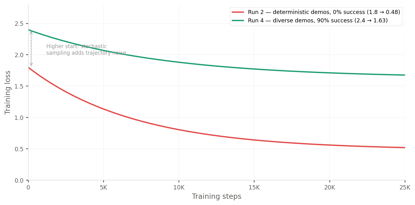
diversity with quantity is gold: the fourth run (third run was an irrelevant run where i tried changing the normalisation to not use mean but only standard deviation but that failed miserably) used 300 episodes collected with deterministic=False which meant SAC would sample from its action distribution instead of taking the mean, so the same target gets different approach angles and timings. the loss settled at 1.63 which is much higher but to my surprise, lead to 90% success! (9 out of 10).
the model that “fit the data worse” performed dramatically better. 0.48 loss meant the diffusion head converged to a tight prediction for each target which signalled memorization. 1.63 loss meant it was fitting a wider distribution of trajectories. now for the same target it actually had to look at the image and figure out what steps to take instead of overfitting to one trajectory. this was the single biggest unlock in the entire pipeline.
realised through trial and error that training loss can’t be an eval metric. a lower loss on memorizable data is worse than a higher loss on diverse data. if your model’s loss is suspiciously low and it’s still failing at the task, check whether it’s memorizing instead of generalizing.
numbers
| method | params | input | training | success | avg steps |
|---|---|---|---|---|---|
| SAC (model-free RL) | 78K | state vector (20 floats) | 300K env steps | 100% | ~95 |
| Octo zero-shot | 93M | image (overhead) | 0 (pre-trained) | 0% | — |
| Octo fine-tuned | 93M | image (overhead + wrist) | 25K ft steps | 90% | ~60 |
the eval loop for the fine-tuned model was to render both cameras, feed to octo, take the first action from the 4-action chunk, apply it, check distance:
for step in range(MAX_STEPS):
    overhead_img = overhead_renderer.render(env.data)
    wrist_img = wrist_renderer.render(env.data)
    img_input = np.asarray(overhead_img, dtype=np.uint8)[np.newaxis, np.newaxis, ...]
    wrist_input = np.asarray(wrist_img, dtype=np.uint8)[np.newaxis, np.newaxis, ...]

    # get action from fine-tuned octo
    actions = model.sample_actions(
        observations={
            "image_primary": img_input,
            "image_wrist": wrist_input,
            "timestep_pad_mask": np.array([[True]], dtype=bool),
        },
        tasks=model.create_tasks(texts=["reach the green target"]),
        rng=sub_rng,
    )

    # actions shape: (1, 4, 7) — use first action from chunk
    raw_action = np.array(actions[0, 0])
    joint_delta = raw_action * action_std + action_mean

    new_qpos = obs["joint_pos"] + joint_delta
    obs = env.step(new_qpos)

    if obs["dist"] < SUCCESS_DIST:
        break
per-episode breakdown from the final run:
| episode | start dist | result | steps |
|---|---|---|---|
| 1 | 0.163m | SUCCESS | 58 |
| 2 | 0.199m | SUCCESS | 62 |
| 3 | 0.107m | SUCCESS | 69 |
| 4 | 0.193m | SUCCESS | 75 |
| 5 | 0.147m | SUCCESS | 59 |
| 6 | 0.101m | SUCCESS | 42 |
| 7 | 0.072m | SUCCESS | 24 |
| 8 | 0.143m | TIMEOUT | 200 |
| 9 | 0.198m | SUCCESS | 156 |
| 10 | 0.127m | SUCCESS | 53 |
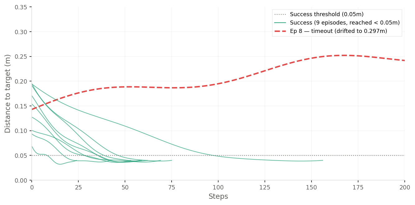
episode 7 started closest and reached in 24 steps. episode 9 was slow but got there. episode 8 started at 0.143m and drifted to 0.297m — a specific target angle where the model didn’t have enough demo coverage. the 10% failure isn’t random, it’s a coverage gap.
one thing i didn’t expect was that octo reaches targets faster (60 steps average) than SAC (95 steps) despite the lower success rate. the action chunking probably helps as 4 jointly-generated actions produce smoother trajectories than SAC’s step-by-step deltas, so less corrective oscillation on approach.
the tradeoff is inference speed. SAC runs in under 1ms on CPU as it’s a tiny MLP. octo takes ~1.5 seconds per step on CPU because you’re running a 93M parameter transformer forward pass plus 20 diffusion denoising iterations which means that real time control would need a GPU.
what actually transferred
while working on this experiment three things were out of distribution for the VLA simultaneously:
visual domain. octo was pre-trained on 800K frames from real cameras which included natural lighting, real textures, real depth. i gave it flat MuJoCo renders with cartoonish colors and no textures. the visual gap between a real franka in a lab and a simulated franka in MuJoCo is very different.
action space. the pretrained action head understood end-effector deltas which is move the gripper by (dx, dy, dz), rotate by some amount, open or close. i threw that away and replaced it with a head that outputs joint angle deltas. the new head was initialized randomly isntead of a trained action head which had knowledge about 800K demonstrations
task and data source. octo’s training data is real teleoperated manipulation. humans moving robot arms to grasp cups, open drawers, push objects on tables. i gave it a floating green sphere in empty space with demonstrations from an RL policy, not a human.
what survived the gap: spatial reasoning. the backbone learned something like “there is a salient object in the scene, the instruction references it, it is in that direction” from seeing 22 different robots interact with objects across 800K trajectories. the concept of spatially locating a target and understanding instructions to go towards it transferred really well to MuJoCo renders. the fine-tuning taught the model what our specific images look like and what our specific action space means. the pre-trained backbone handled the perceptual heavy lifting that made 300 demos sufficient.
what didn’t survive: action knowledge. zero-shot eval was 0%. the arm drifted away from the target every episode. the pre-trained head’s understanding of end-effector control was meaningless in joint angle space. the new diffusion head learned entirely from our 300 demonstrations, starting from random weights.
this lines up with what the octo paper hypothesized. their architecture was designed around the idea that cross-embodiment transfer works if you separate what transfers (visual reasoning in the backbone) from what doesn’t (motor commands in the action head). the invisible readout token means swapping the head preserves the backbone’s representations exactly. and fine-tuning the backbone with a small learning rate lets it adapt to the new visual domain without destroying what it learned from 800K demos.
what i find interesting is how far this stretched. octo was designed for fine-tuning on a new real robot with real cameras and a different end-effector. i gave it synthetic renders, a completely different action parameterization, and RL-generated demos instead of teleoperation. three gaps at once, all outside the intended use case. and the backbone’s spatial reasoning still carried enough signal for 90% success with 300 demos and 47 minutes of fine-tuning.
93M parameters is small by current standards. pi0 is 3B. openVLA is 7B. if positive transfer works at this scale with this many domain gaps, larger models trained on more diverse data should do better. the pretrained backbone was fundamental as otherwise, 30K sim demos alone would never teach both vision and control from scratch. the fine-tuned checkpoint is available on huggingface if you want to verify or build on this.
what’s next
harder tasks: pick-and-place, multi-step manipulation — where the backbone’s pre-trained visual understanding should matter more than it does for simple reaching real-world transfer: 3D-print a robot arm, mount a real camera, mix sim and real data, fine-tune a larger VLA like pi0 or openVLA on actual hardware