building and breaking llms from scratch
tech ·i’ve always treated llms as blackbox which help me build non-determinstic workflows in code (read ai agents). attention heads, layernorms, transformers, topk, temperature, feed forward networks, all of these were just buzzwords which i had faint ideas about as i was just using hosted llm inference apis to get the job done but i always wanted to know what’s inside, how data flows, how decisions are made and how each layer affects each other and the whole “gpt” as a whole
decided to build the entire thing from scratch, the embedding layer, the multi-headed causal attention class, the feedforward network, and attach all of these with layernorms and residual connections all together in a neat transformer block. i also decided to pretrain the transformer using tinystories data set on hugging face (massively undertrained) and then added instrumentation to see the actual attention weights during inference time and how they behave. added ablators to remove some attention heads, some attention layers all together and even mlp layers to see how the model would perform. got some interesting findings out of this analysis which i’ll write about as well
a lot of how i built the transformer is inspired by sebastian raschka’s book - building an llm from scratch. special mention because that is what got me poking around and getting an intuitive understanding about llms. the breaking part is something i tinkered around without prior learning. mechanistic interpretability was a totally new concept before i started the project and model hooks, ablations and layer level study is something which got me a real solid sense about internal workings and got me some good insights as well
the post is both a summarisation dump for myself, and hopefully an easy helpful reading for someone getting into building llms and wanting to get a picture a level deep inside transformer architecture and how internal layers work to give you the gpt answer you prompt for
we break it down into 4 phases, building the transformer (embeddings, attention, mlp block, full gpt), training (downloading and prepping the dataset, building the training loop, generating text from the trained transformer), breaking and analyzing the transformer (instrumentation, ablations and analysis) i recommend you feed this blog post to claude or gpt and keep asking questions to fill your knowledge gap wherever required
in case you want to dive directly into the code
building the llm
the llm is a repeated sequence of attention and mlp blocks sequenced together with layernorms and residual connections all together forming the transformer block. most of the computation inside these different terminologies is just multiplications done between different weight matrices
i wont go into extreme depth of each terminology otherwise this blog post will become a 500 page long book but i will give broad enough idea so that a bigger picture can be seen on how different things are joined together
i want some constants handy throughout the build so i will first create a dataclass called GPTConfig which will store these values for me
i will quickly give a one liner on some terms that will be used
vocab_size: the number of unique tokens in the vocabulary. think of this as the global lookup table from which we get the token_id of each word. “banana” has a token_id of 12345 - we get to know this by looking up the word in the vocabulary and getting the index.
context_length: this is the length of sequence of tokens the model will be able to process at a time. for the small model that we’re training we’re keeping it to be 512 but for a world class gpt 5 model this could be 100k tokens or more
n_layers: the number of transformer blocks in the model, we will use 6 for our usecase
n_heads: we build a multi-headed causal attention mechanism which requires us to split the attention matrix into multiple heads each specialising in a different kind of relationship between tokens (syntactic, semantic, positional, long range dependency) - just know that the attention matrix will be split into multiple heads in our case - 6
d_model: this is the dimension of the vectors that would represent each token. the higher the dimensions, the granular the point in space for that token to be represented. we use a dimension of 384 for our model (keep it divisible by the n_heads parameter because the dimension gets split into heads during attention)
d_ff: this is the dimension of the feedforward network. how big of a feature space we want the activations to go through is defined by this
dropout: we randomly make certain values in our attention weights zero to prevent overfitting, removing deterministic relations between words/tokens
bias: we don’t use this and set it to False. it’s basically to add some bias values to the matrix after doing linear transformations
from dataclasses import dataclass

@dataclass
class GPTConfig:
    vocab_size: int = 50257
    context_length: int = 512
    n_layers: int = 6
    n_heads: int = 6
    d_model: int = 384
    d_ff: int = 1536
    dropout: float = 0.1
    bias: bool = False

    def __post_init__(self):
        assert self.d_model % self.n_heads == 0, \
            f"d_model {self.d_model} must be divisible by n_heads {self.n_heads}"

    @property
    def d_head(self) -> int:
        return self.d_model // self.n_heads
we will also add a helper here in the config file to help us give an estimated number of parameters that will be active/used in the model
def estimate_params(self) -> int:
    token_emb = self.vocab_size * self.d_model
    pos_emb = self.context_length * self.d_model

    attn = 4 * self.d_model * self.d_model  # Q, K, V, O projections
    mlp = self.d_model * self.d_ff + self.d_ff * self.d_model  # expand + contract
    ln = 2 * self.d_model  # scale (gamma) + shift (beta) params

    per_block = attn + mlp + ln
    final_ln = self.d_model

    return token_emb + pos_emb + self.n_layers * per_block + final_ln
this is basically the number of values that get stored. we have an embedding matrix, a positional embedding matrix, an attention module which contains 4 matrices, mlp which contains an upward and downward projection and gelu, and layernorms (shift and scale params) that we apply to each layer. now we have 6 layers so we multiply this and then add a final layer norm
we get a ~30M parameter model with the config we have. there is a concept of weight tying which we use which doesn’t require us to store the output projection matrix because it is the same as the embedding matrix but not going into detail there
the embedding layer
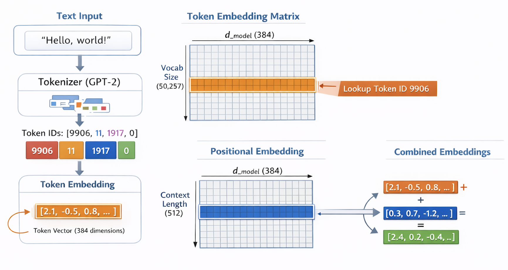
the input that gets fed into a prompt is a string, the model understands numbers. this concept is same during inference and training. we need to convert the stream of inputs into the model recognisable token ids which then get a vector representation called an embedding.
we create a tokenizer which is nothing but a wrapper around the tiktoken tokeniser. we initialise the tokeniser using gpt2 tokenisation scheme which means that the vocabulary we earlier talked about which would contain the word and its corresponding token would be defined here. we also get a pretrained tokeniser which knows how gpt splits text and we will use the same splitting technique (byte pair encoding). BPE helps tokenise unknown words well just know that
example
tokenizer = Tokenizer("gpt2")  # Uses GPT-2's encoding scheme
text = "Hello, world!"
tokens = tokenizer.encode(text)  # [9906, 11, 1917, 0] (example IDs)
now coming to the embedder which receives these token_ids - this is the first layer of the model which stores a trainable matrix. it is a matrix of shape [vocab_size, d_model] which basically acts as a lookup table assigning the token id to its corresponding vector. we also store another matrix called positional embeddings which is of shape [context_length, d_model]. it stores the positional information about a token. it adds value to the token embedding based on which position/index it is in the sequence. this helps differentiate between the word “break” in “I need a break” and “I had a break up”. we also add a dropout (zero random values in the matrix, to prevent overfitting - encourages the model to not form strong relations early and use distributed features instead of overweighted dimensions of the embeddings)
class Embedding(nn.Module):
    """Convert token ids to vectors and add positional information."""

    def __init__(self, config: GPTConfig):
        super().__init__()
        self.token_embedding = nn.Embedding(config.vocab_size, config.d_model)
        self.positional_embedding = nn.Embedding(config.context_length, config.d_model)
        self.dropout = nn.Dropout(config.dropout)

    def forward(self, token_ids):
        """
        Input: (batch, seq_len) - integer token IDs
        Output: (batch, seq_len, d_model) - embedding vectors
        """
        token_embeddings = self.token_embedding(token_ids)
        positional_embeddings = self.positional_embedding(
            torch.arange(token_ids.size(1), device=token_ids.device)
        )
        embeddings = token_embeddings + positional_embeddings
        embeddings = self.dropout(embeddings)
        return embeddings
in pytorch, inheriting from nn.Module registers layers and parameters, tracks gradients and calls forward() when we use the model. it helps connect all our layers into a trainable neural network
the attention layer
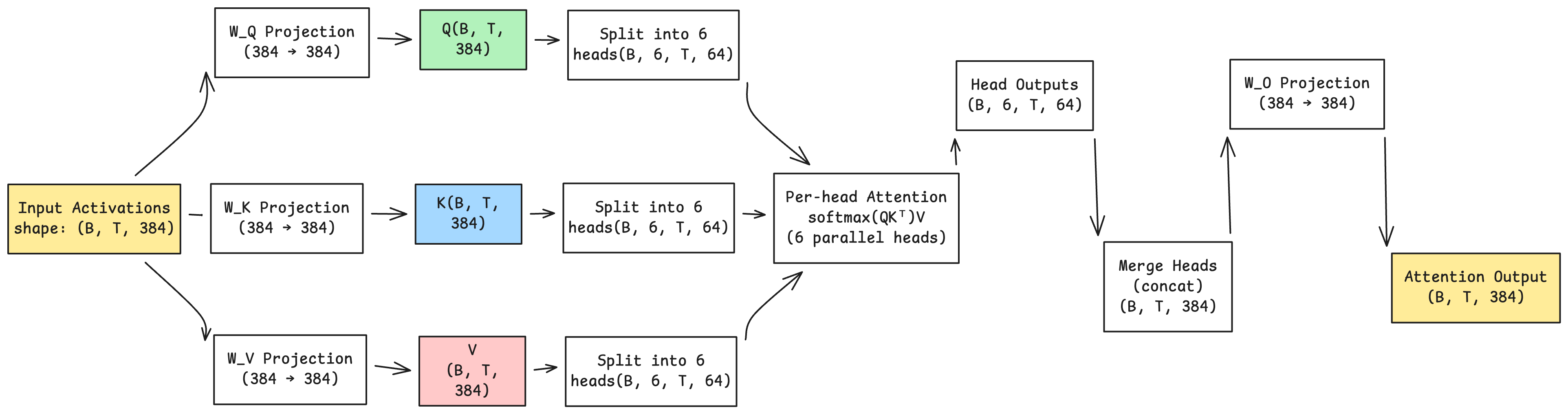
this is the first magical piece of the transformer. it is a series of actions taken for all tokens which allows all the tokens to have contextual information about each other. the repeatable process on top of which attention is built is - for each token in a sequence we calculate the distance of that token with every other token using a dot product between the token vectors, these become the attention scores ie how closely or further related in the multidimensional space the tokens are. then softmaxing the attention scores into attention weights and doing a weighted sum of all the tokens with their attention weights. this would be the context vector for the token we are comparing against. now imagine doing this for all vectors.
for this we maintain a few weights - query, key and value projection matrices. the key matrix can be seen as the matrix which is used as input matrix to calculate attention weights. the query matrix can be seen as comparing to each token of the key matrix but for all tokens so it becomes a matrix. the value matrix is what we do the weighted sum by referencing the attention weights
this is what we’re going to build
\[\text{Attention Weights} = QK^\top\] \[\text{Output} = \text{softmax}(QK^\top)V\]where $Q$ is the queries matrix, $K$ is the keys matrix, and $V$ is the values matrix. finally, we apply a linear (output) projection to the result.
note that we are doing causal attention which means that we are not allowing a token to see the future tokens in the sequence. this is a key feature of the transformer architecture and is what allows it to process historical sequence data in parallel.
scores = scores.masked_fill(self.causal_mask[:T,:T] == 0, float('-inf'))
when we apply the mask so that positions in the upper diagonal are set to $-\infty$, the softmax over a row $i$ looks like:
\[\text{softmax}(s_i)_j = \frac{\exp(s_{ij})}{\sum_{k=1}^{T} \exp(s_{ik})}\]if $s_{ij} = -\infty$ for $j > i$ (future tokens), then $\exp(-\infty) = 0$, so those terms contribute nothing. thus, for each token $i$, attention weights to all tokens $j > i$ become zero:
\[\text{softmax}(s_{ij} = -\infty) = 0\ \text{for}\ j > i\]this enforces that each token can only attend to itself and previous tokens in the sequence.
the other concept here is multi headed attention where we actually split the attention matrices into 6 different parts which get processed simultaneously. why multi-head? each head can specialise in learning different kinds of relationships - syntactic, semantic, positional, long range dependencies. instead of one attention mechanism trying to capture everything, we get 6 parallel specialists.
note that the shape of the initial attention projection matrices is [d_model, d_model], which means the Q,K,V matrices will be projections of the input with shape [batch, context_length, d_model]. we need to split this into heads
# we split 384 into 6 heads of 64 dimensions each
# b,t,384 -> b,t,6,64 -> b,6,t,64 (transpose for parallel work)
Q = Q.view(B, T, self.n_heads, self.d_head)
Q = Q.transpose(1,2)  # now heads dimension is before sequence
after computing attention for all heads in parallel, we reassemble them back:
# b,6,t,64 -> b,t,6,64 -> b,t,384
output = output.transpose(1,2)
output = output.contiguous().view(B, T, C)
output = self.W_O(output)  # final output projection
the .contiguous() call is needed because transpose creates a non-contiguous tensor in memory. view needs contiguous memory layout to work
this is how the attention class looks like:
class CausalSelfAttention(nn.Module):
    def __init__(self, config: GPTConfig):
        super().__init__()
        self.W_Q = nn.Linear(config.d_model, config.d_model, bias=config.bias)
        self.W_K = nn.Linear(config.d_model, config.d_model, bias=config.bias)
        self.W_V = nn.Linear(config.d_model, config.d_model, bias=config.bias)
        self.W_O = nn.Linear(config.d_model, config.d_model, bias=config.bias)

        self.register_buffer("causal_mask", torch.tril(torch.ones(config.context_length, config.context_length)))
        self.dropout = nn.Dropout(config.dropout)
        self.n_heads = config.n_heads
        self.d_head = config.d_head

    def forward(self, x):
        B, T, C = x.shape

        # project and split into heads
        Q = self.W_Q(x).view(B, T, self.n_heads, self.d_head).transpose(1,2)
        K = self.W_K(x).view(B, T, self.n_heads, self.d_head).transpose(1,2)
        V = self.W_V(x).view(B, T, self.n_heads, self.d_head).transpose(1,2)

        # scaled dot-product attention with causal mask
        scores = Q @ K.transpose(-2,-1) / math.sqrt(self.d_head)
        scores = scores.masked_fill(self.causal_mask[:T,:T] == 0, float('-inf'))
        attention_weights = F.softmax(scores, dim=-1)
        attention_weights = self.dropout(attention_weights)

        # weighted sum of values
        output = attention_weights @ V

        # reassemble heads and project
        output = output.transpose(1,2).contiguous().view(B, T, C)
        output = self.W_O(output)
        output = self.dropout(output)
        return output
we apply dropout twice - once on attention weights (prevents overfitting to specific token relationships) and once on output (prevents overfitting to specific feature dimensions)
the mlp block
while attention lets tokens “talk” to each other and share information, the mlp processes each token independently. think of it as feature extraction and transformation at each position. the expanded dimensions act as feature storage columns for information about the token. the mlp processes the tokens sequentially unlike attention which processes the token and all the tokens behind it parallelly
the architecture expands the dimension from d_model (384) to d_ff (1536) - 4x expansion, then applies GELU activation (non-linearity), then compresses back to d_model (384)
why expand then compress? the expanded space gives the network more capacity to learn complex transformations. it’s like giving yourself more working space before consolidating information into original dimensions
GELU (Gaussian Error Linear Unit) adds non-linearity to the network, but does so in a smoother way than ReLU.
ReLU simply sets all negative values to zero: f(x) = max(0, x). this creates a hard cutoff at zero, which can lead to sharp gradient changes during backpropagation (the gradient is either 0 or 1, with a discontinuity at x=0).
GELU instead uses a smooth, probabilistic approach. the mathematical formula is:
GELU(x) = x · Φ(x)
where Φ(x) is the cumulative distribution function of the standard normal distribution. this function smoothly scales the input based on how “positive” it is - values that are more negative get scaled down more, while positive values pass through more fully. think of it as softly “gating” the information rather than making a hard cut. this smoothness leads to more stable gradients during training which means activation smoothly transitions rather than having an abrupt jump at zero.
class MLP(nn.Module):
    def __init__(self, config: GPTConfig):
        super().__init__()
        self.W_1 = nn.Linear(config.d_model, config.d_ff, bias=config.bias)  # expand
        self.W_2 = nn.Linear(config.d_ff, config.d_model, bias=config.bias)  # contract
        self.dropout = nn.Dropout(config.dropout)

    def forward(self, x):
        x = self.W_1(x)      # expand: (batch, seq, 384) -> (batch, seq, 1536)
        x = F.gelu(x)        # non-linearity
        x = self.W_2(x)      # contract: (batch, seq, 1536) -> (batch, seq, 384)
        x = self.dropout(x)
        return x
an important thing to note is that attention mixes information across tokens (token-to-token relationships), mlp transforms features at each position independently (no cross-token communication)
the transformer block
now we combine attention and mlp together with two crucial additions: layer normalisation and residual connections
layer normalisation: during backpropagation, gradients flow through many multiplications because of chain rule of differentiation. without normalisation, these can explode (become huge) or vanish (become tiny). layernorm squishes activations to have mean=0 and variance=1 at each layer, keeping gradients stable
layer norm also has two trainable parameters - scale and shift. after normalizing to mean=0 and variance=1, these parameters allow the model to adjust the distribution if needed. the formula is: output = scale * normalized_input + β. if the model learns that mean=0 and variance=1 isn’t optimal for that layer, it can use scale and shift to transform the activations to a better distribution while still maintaining gradient stability from the normalization step.
residual connections: instead of output = block(x), we do output = x + block(x). the original input is added back to the output, creating a “gradient highway”—even if the block learns nothing useful, gradients can still flow directly through that addition.
the chain rule for this is:
\[y = x + \mathrm{block}(x)\]so,
\[\frac{\partial\, \mathrm{Loss}}{\partial x} = \frac{\partial\, \mathrm{Loss}}{\partial y} \left( \frac{\partial\, \mathrm{block}(x)}{\partial x} + \frac{\partial x}{\partial x} \right)\]since $\frac{\partial x}{\partial x}$ is just the identity matrix…
\[\frac{\partial\, \mathrm{Loss}}{\partial x} = \frac{\partial\, \mathrm{Loss}}{\partial y} \left( \text{block gradient} + I \right)\]this lets the identity matrix flow and prevents gradients from vanishing entirely
we use pre-norm architecture (GPT-2 style) where layernorm is applied before each sub-block, not after:
x = x + attention(layernorm(x))  # not: layernorm(x + attention(x))
x = x + mlp(layernorm(x))
why pre-norm? let’s compare the gradient paths. with post-norm (layernorm after the residual), the gradient flow goes: loss -> layernorm -> (residual connection + block output). both paths (the residual shortcut and the block) must go through layernorm. if layernorm’s gradients are problematic, both paths are affected.
with pre-norm (layernorm before the block), the gradient flow goes: loss → (residual connection directly + block → layernorm). the residual connection creates a direct path that bypasses layernorm entirely. the gradient along the residual path is simply 1 (since ∂x/∂x = 1), with no scaling or transformation. only the block’s output passes through layernorm.
this direct gradient highway means that even if the block and layernorm struggle to pass gradients, the residual connection ensures gradients always flow through. this stability allows us to use higher learning rates right from the start of training, without needing a “warmup period” (where you gradually increase the learning rate from a small value to the target value over many steps).
we will discuss what learning rate is later
class TransformerBlock(nn.Module):
    def __init__(self, config: GPTConfig):
        super().__init__()
        self.ln_1 = nn.LayerNorm(config.d_model)
        self.attention = CausalSelfAttention(config)
        self.ln_2 = nn.LayerNorm(config.d_model)
        self.mlp = MLP(config)

    def forward(self, x):
        x = x + self.attention(self.ln_1(x))  # attention + residual
        x = x + self.mlp(self.ln_2(x))        # mlp + residual
        return x
the flow is: input → layernorm → attention → add back input → layernorm → mlp → add back → output
think of residual connections as accumulation as a safety measure whenever each block adds new information to the stream rather than replacing what was there
the full gpt model
now we stack everything together: embedding layer (token + positional), 6 transformer blocks, final layer normalisation, and output projection to vocabulary size
class GPT(nn.Module):
    def __init__(self, config: GPTConfig):
        super().__init__()
        self.config = config
        self.embedding = Embedding(config)
        self.blocks = nn.ModuleList([TransformerBlock(config) for _ in range(config.n_layers)])
        self.ln_f = nn.LayerNorm(config.d_model)
        self.W_O = nn.Linear(config.d_model, config.vocab_size, bias=False)

        # weight tying - share embedding and output weights
        self.W_O.weight = self.embedding.token_embedding.weight

    def forward(self, x):
        x = self.embedding(x)           # (batch, seq) -> (batch, seq, d_model)
        for block in self.blocks:
            x = block(x)                # (batch, seq, d_model) -> same
        x = self.ln_f(x)                # final normalisation
        logits = self.W_O(x)            # (batch, seq, d_model) -> (batch, seq, vocab_size)
        return logits
a few things to note:
nn.ModuleList is required instead of a regular python list - it registers all the block parameters so pytorch knows to train them
weight tying: we share weights between the token embedding matrix and the output projection. both are shape (vocab_size, d_model). embedding maps token_id → vector, output projection maps vector → logits. mathematically similar operations, so sharing saves ~19M parameters. when one updates during training, the other updates too
the output logits are unnormalised scores for each possible next token. the final activations from the last transformer block (shape: batch, seq_len, d_model) are projected through a linear layer into vocabulary space, producing logits with shape (batch, seq_len, vocab_size). this means for each position in each sequence, we get 50,257 raw scores - one for each token in the vocabulary.
to predict the next token, we apply softmax to the logits to convert them into probabilities (so they sum to 1), then select the token with the highest probability. for example, if token 1234 (representing “banana”) has the highest probability after softmax, that becomes the predicted next token. [can attach an image here]
training the model
now that we’re done with the skeleton its time to feed it some patterns to recognise. we need data, a training loop, and a way to generate text from the trained model
the dataset
we use tinystories from huggingface - a dataset of simple children’s stories. perfect for training a small model because the language patterns are simpler than wikipedia or web text, and this would work for our ablation study. we download stories from huggingface, tokenise all stories into one long stream of tokens, then chunk into fixed-length sequences of context_length (512)
the first time the dataset will take some time to download post which it will be stored in cache, huggingface has train and validation sets mentioned that we can automatically split the data by.
we have a max_examples parameter which we can use if we quickly want to load and not wait for training all the data.
this is how the dataset class looks like:
class TinyStoriesDataset(Dataset):
    def __init__(self, split="train", context_length=512, max_examples=None):
        self.context_length = context_length
        self.tokenizer = Tokenizer()
        self.dataset = load_dataset("roneneldan/TinyStories", split=split)

        # concatenate all stories into one token stream
        all_tokens = []
        for i, example in enumerate(self.dataset):
            if max_examples and i >= max_examples:
                break
            tokens = self.tokenizer.encode(example['text'])
            all_tokens.extend(tokens)

        # chunk into fixed-length sequences
        self.examples = []
        for i in range(0, len(all_tokens) - context_length, context_length):
            chunk = all_tokens[i:i+context_length]
            self.examples.append(chunk)

    def __len__(self):
        return len(self.examples)

    def __getitem__(self, idx):
        return torch.tensor(self.examples[idx], dtype=torch.long)
the __len__ and __getitem__ methods are required for pytorch’s DataLoader which handles batching and shuffling automatically. DataLoader shuffles indices not actual data - much more memory efficient
the training loop
training a language model is next-token prediction. given tokens [0:n-1], predict token [n]. we do this for every position in the sequence for each sequence in a batch of sequences.
# split batch into input and target
input = batch[:, :-1]   # all but last token
target = batch[:, 1:]   # all but first token
for sequence “the cat sat”, input is “the cat”, target is “cat sat”. we’re predicting each next token given everything before it
loss function: cross-entropy loss. let me break this down because it took me a while to get an intuition for it
we have logits - raw scores for each of the 50,257 vocabulary tokens. softmax converts these into probabilities (sum to 1). now for each position, we know the actual next token from our training data.
say the correct next token is “cat” at vocabulary index 2345. after softmax, we look at position 2345 in our probability distribution. ideally, this should be 1.0 (100% confident it’s “cat”). in practice it’s something like 0.3 or 0.7.
cross-entropy loss = -log(probability of correct token)
why negative log? if probability = 1.0, then -log(1.0) = 0 → perfect prediction, zero loss. if probability = 0.5, then -log(0.5) ≈ 0.69 → uncertain, some loss. if probability = 0.01, then -log(0.01) ≈ 4.6 → wrong prediction, high loss.
the log makes small probabilities punishing (exponentially so) and the negative flips it so lower is better. we’re essentially asking: “how surprised was the model by the correct answer?” low probability = high surprise = high loss
we compute this for every position in every sequence and average it all. so if batch is (8, 512), we’re averaging across 8 × 511 = 4088 next-token predictions per batch
def compute_loss(self, batch):
    input = batch[:, :-1]
    target = batch[:, 1:]
    logits = self.model(input)

    # flatten for cross_entropy: (batch, seq, vocab) -> (batch*seq, vocab)
    logits_flat = logits.contiguous().view(-1, logits.size(-1))
    targets_flat = target.contiguous().view(-1)

    loss = F.cross_entropy(logits_flat, targets_flat)
    return loss
the .contiguous().view() pattern appears again - this is because slicing into inputs and targets slicing creates non-contiguous tensors, which we need to fix that before reshaping. we can also use .reshape() which handles this internally
optimiser: AdamW with learning_rate=3e-4 and weight_decay=0.1. let me break down what’s actually happening during optimization because it took me a while to understand the mechanics
when we call loss.backward(), pytorch computes gradients which are the derivative of loss with respect to every model parameter. these gradients are stored in each parameter’s .grad attribute. so if you have a weight matrix W in a linear layer, after backward pass you’ll have W.grad containing how much each weight contributed to the loss
the basic idea of optimization is that if a weight’s gradient is positive, that weight increased the loss, so we should decrease it. if gradient is negative, the weight decreased loss, so we should increase it. we move weights in the opposite direction of the gradient
vanilla SGD (stochastic gradient descent) does this simply
\[w_{new} = w_{old} - \alpha \cdot \frac{\partial L}{\partial w}\]where $\alpha$ is the learning rate (how big steps we take) and $\frac{\partial L}{\partial w}$ is the gradient. this works but has problems: same learning rate for all parameters (some might need bigger/smaller steps), no memory of past gradients (oscillates), and can get stuck in flat regions
Adam (adaptive moment estimation) fixes this with two innovations. first, momentum - keeps track of past gradients to smooth out updates. instead of using just the current gradient, we use a running average:
\[m_t = \beta_1 \cdot m_{t-1} + (1 - \beta_1) \cdot g_t\]where $m_t$ is the momentum at step $t$, $g_t$ is current gradient, and $\beta_1$ (typically 0.9) controls how much we remember past gradients
second, adaptive learning rates - each parameter gets its own learning rate based on how much it’s been updated. parameters with large gradients get smaller learning rates, parameters with small gradients get larger ones:
\[v_t = \beta_2 \cdot v_{t-1} + (1 - \beta_2) \cdot g_t^2\] \[w_{new} = w_{old} - \alpha \cdot \frac{\hat{m}_t}{\sqrt{\hat{v}_t} + \epsilon}\]where $v_t$ tracks the variance of gradients, $\hat{m}_t$ and $\hat{v}_t$ are bias-corrected versions (to account for initialization), and $\epsilon$ (typically 1e-8) prevents division by zero
AdamW (Adam with weight decay) adds weight decay properly. in regular Adam, weight decay gets mixed with gradient updates. AdamW decouples it:
\[w_{new} = w_{old} - \alpha \cdot \frac{\hat{m}_t}{\sqrt{\hat{v}_t} + \epsilon} - \lambda \cdot w_{old}\]where $\lambda$ is weight_decay (0.1 in our case). this separately pulls weights toward zero, acting as L2 regularization (punishment for large weights). it’s like gravity after the learning rate helps weights jump around to find good values, weight decay gently pulls them back toward zero to prevent overfitting
why weight_decay=0.1? it’s a hyperparameter that controls regularization strength. too high and weights get pulled too hard toward zero (underfitting). too low and model might overfit. 0.1 is a common default that we have used
the learning_rate=3e-4 (0.0003) is also empirically proven to work well for GPT-style models. it’s small enough to avoid overshooting but large enough to make progress. with pre-norm architecture we can use this from the start without warmup
when we call optimiser.step(), all these formulas are applied to every parameter in the model. then optimiser.zero_grad() clears the gradients so they don’t accumulate across batches
class Trainer:
    def __init__(self, model, train_dataloader, val_dataloader=None,
                 learning_rate=3e-4, weight_decay=0.1, device="mps"):
        self.model = model.to(device)
        self.optimiser = AdamW(model.parameters(), lr=learning_rate, weight_decay=weight_decay)

    def train_epoch(self):
        self.model.train()  # enable dropout
        for batch in self.train_dataloader:
            batch = batch.to(self.device)
            loss = self.compute_loss(batch)
            loss.backward()         # compute gradients
            self.optimiser.step()   # update weights
            self.optimiser.zero_grad()  # clear gradients for next batch

    def validate(self):
        self.model.eval()  # disable dropout
        with torch.no_grad():  # don't track gradients during validation
            # compute validation loss...
model.train() vs model.eval() - training mode enables dropout, eval mode disables it. during inference we want the full model, not randomly zeroed values
we also checkpoint after each epoch / each training run - save model weights and optimiser state so we can resume training or load for inference later. ideally we should keep running training loops / epochs till we find the minimum loss value for the model, but here we ran two epochs, collected information, analysed layers and then ran two more epochs to validate a hypothesis
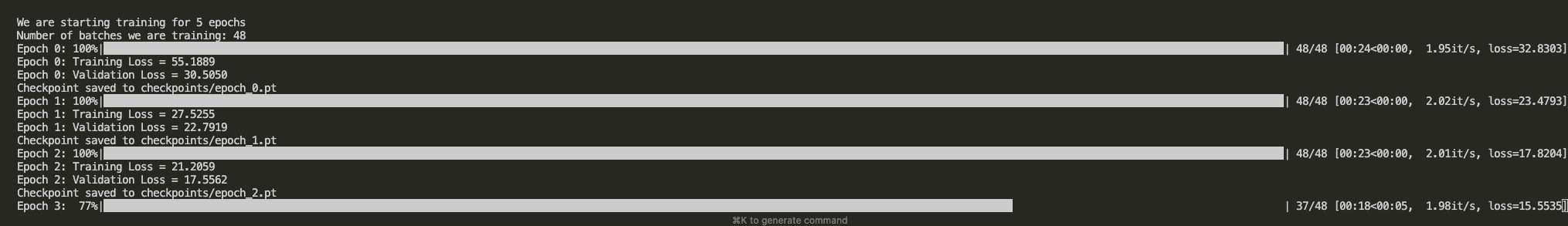
it/s is number of batches that gets processed per second (this is for mac’s mps)
text generation
now we have a trained transformer which has learned some of the patterns in the tiny stories dataset. we used 500 max examples for training to get a model up and running.
now that training is done, the model can generate text autoregressively - one token at a time, feeding each prediction back as input for the next
class Generator:
    def __init__(self, config, model, tokenizer, device):
        self.model = model.to(device)
        self.model.eval()  # inference mode
        self.tokenizer = tokenizer

    def generate(self, prompt, max_tokens=50, temperature=1.0, top_k=None):
        tokens = self.tokenizer.encode(prompt)
        tokens = torch.tensor(tokens).unsqueeze(0).to(self.device)  # add batch dim

        with torch.no_grad():
            for _ in range(max_tokens):
                # truncate if exceeds context length
                if tokens.size(1) > self.config.context_length:
                    tokens = tokens[:, -self.config.context_length:]

                logits = self.model(tokens)
                last_logits = logits[:, -1, :]  # only care about last position

                # temperature scaling
                scaled_logits = last_logits / temperature

                # top-k filtering (optional)
                if top_k:
                    values, _ = torch.topk(scaled_logits, top_k)
                    min_val = values[:, -1].unsqueeze(-1)
                    scaled_logits = torch.where(
                        scaled_logits < min_val,
                        float('-inf'),
                        scaled_logits
                    )

                probs = F.softmax(scaled_logits, dim=-1)
                next_token = torch.multinomial(probs, num_samples=1)
                tokens = torch.cat([tokens, next_token], dim=1)

        return self.tokenizer.decode(tokens.squeeze(0).tolist())
tokens = torch.tensor(tokens).unsqueeze(0).to(self.device) converts the input tokens into a batched prompt tensor which can be fed to the transformer network we created
unlike training where we cared about logits for all tokens while computing loss, during inference, we only care about the last logits, because the last token has attention from all the previous tokens
before converting the logits into probability we apply two post generation optimisations to choose the best next token:
temperature: dividing logits by temperature before softmax. temperature > 1.0 makes the distribution more uniform (more random/creative). temperature < 1.0 makes it sharper (more deterministic/repetitive)
if a particular logit has a spike i.e it is most likely to be predicted as next token, a higher temperature would normalise it to behave less spiky, whereas a lower temperature would further increase the spike making it stand out
top-k filtering: out of the 50257 possible selections for the next token, if we just want to select from the top k samples with the highest logit values, we can reduce the number of tokens to consider. prevents the model from occasionally outputting nonsense low-probability tokens
torch.topk gives the top k values with their indices in descending order. we dont care about the indices. we get the minimum value out of the list of top k and broadcast it to the same shape as the logits to compare each logit against the min_value and replace it by negative infinity before it goes to softmax (a similar concept we used for the causal mask where we make the value -inf so that softmax makes it 0)
torch.multinomial samples from the probability distribution - we don’t always pick argmax (highest probability). this adds randomness and variety to generation
this way, the model doesn’t deterministically output the same thing everytime, but instead samples from the probability distribution to give a more natural varied output
example
from src.model.config import GPTConfig
from src.model.transformer import GPT
from src.data.tokenizer import Tokenizer
from src.generation.generator import Generator

# load trained model
config = GPTConfig()
model = GPT(config)
checkpoint = torch.load("checkpoints/epoch_4.pt", map_location="mps")
model.load_state_dict(checkpoint["model_state_dict"])

# create generator
device = "mps" if torch.backends.mps.is_available() else "cpu"
tokenizer = Tokenizer()
generator = Generator(config, model, tokenizer, device)

# generate text
prompt = "Once upon a time"
output = generator.generate(prompt, max_tokens=50, temperature=1.0)
print(output)
this loads a checkpoint, initializes the generator, and produces text from the prompt. the model continues the story autoregressively till it reaches the max tokens or the model generates the end of sentence token.
breaking the model - instrumentation
we successfully built a transformer from scratch, pretrained it with a small sample of a huggingface dataset, created generation logic to output next tokens for a prompt. now we want to understand that during the process of generating the next token, how do the attention layers look like, what is going on inside - what can the attention weights tell us
for this we will create instrumentation inside the attention blocks. we will do this by using a pytorch functionality called forward hooks which lets us call register_forward_hook on the attention block to capture the attention weights during the forward pass. basically before the attention layer output is relayed forward, we capture the intermediate state.
when we register a forward hook, it acts like a sequential function which gets executed right after the forward pass of the module the forward hook is registered to. the hook receives the module instance the input it received and the output the module produced
we use it to capture attention weights
class Instrumenter:
    def __init__(self, model):
        self.model = model
        self.activations = defaultdict(list)
        self.hooks = []

    def register_attention_hooks(self):
        def make_hook(layer_idx):
            def hook(module, input, output):
                if hasattr(module, 'attention_weights'):
                    key = f"attention_layer_{layer_idx}"
                    self.activations[key].append(
                        module.attention_weights.detach().cpu()
                    )
            return hook

        for i, block in enumerate(self.model.blocks):
            hook_handle = block.attention.register_forward_hook(make_hook(i))
            self.hooks.append(hook_handle)

    def get_attention_weights(self, layer_idx):
        return self.activations[f"attention_layer_{layer_idx}"][0]

    def clear(self):
        self.activations.clear()

    def remove_hooks(self):
        for hook in self.hooks:
            hook.remove()
        self.hooks.clear()
the make_hook closure is needed because we want each hook to remember its layer index. if we didn’t use a closure, all hooks would reference the same i variable (the last value from the loop)
.detach().cpu() is important - we detach from the computation graph (no gradient tracking needed as we are in inference mode) and move to CPU to free GPU memory
attention weights have shape (batch, n_heads, seq_len, seq_len) - that is for each head, we get a square matrix showing how much each token attends to every other token. this is the core interpretability data
with instrumentation we can now analyze what’s happening inside. let me show you what i found when i ran the model on the prompt “once upon a time” (tokenized as [27078, 2402, 257, 640]):
visualizing attention patterns
each attention matrix shows how tokens attend to each other. as our attention layers are split between 6 heads each head would have its own attention matrix. for example this is what a layer 0, head 0 would look like for a forward pass for the transformer we made
layer 0, head 0:
      Tok 0 Tok 1 Tok 2 Tok 3
Tok0: 1.000 0.000 0.000 0.000  (100% self-attention - no past tokens)
Tok1: 0.507 0.493 0.000 0.000  (attends to previous token)
Tok2: 0.285 0.155 0.560 0.000  (attends to self and previous tokens)
Tok3: 0.104 0.279 0.160 0.457  (distributed attention, with max attention to self)
layer 5, head 0:
      Tok 0 Tok 1 Tok 2 Tok 3
Tok0: 1.000 0.000 0.000 0.000
Tok1: 0.498 0.502 0.000 0.000  (more uniform)
Tok2: 0.334 0.337 0.329 0.000  (very uniform)
Tok3: 0.252 0.254 0.247 0.247  (almost equal attention unlike layer 0 head 0 where the attention was concentrated towards self)
we observed that early layers (0-2) show more focused structured patterns where there is more attention to the current token than the previous ones as we move ahead in the transformer blocks, later layers (4-5) become more uniform where attention is spread more evenly across tokens. this kind of gives a hint that later layers spread more uniformity than early layers of attention
another thing to point out here for clarity is that you will notice that token 0 always has 1.000 self-attention in every layer. this is the causal mask in action as the first token has no past tokens to attend to, so it can only attend to itself. this pattern is consistent across all layers and heads, confirming the causal mechanism is working correctly as well!
comparing self and other attention, i measured how much each head focuses on itself (diagonal) vs other tokens (off-diagonal).
self_attention = head.diagonal().mean().item()
other_attention = (head.sum() - head.diagonal().sum()).item() / (head.numel() - head.size(0))
for layer 0: head 0 has 62.7% self-attention, 12.4% other-attention (very self-focused), head 1 has 43.7% self-attention, 18.8% other-attention (more balanced), head 2 has 52.7% self-attention, 15.8% other-attention, head 3 has 50.9% self-attention, 16.4% other-attention, head 4 has 48.9% self-attention, 17.0% other-attention, head 5 has 41.1% self-attention, 19.6% other-attention (most other-focused)
it was interesting to find out that different heads in the same layer specialize differently. head 0 is very self-focused (62.7%) can call it introverted, while head 5 is more other-focused (only 41.1% self-attention) likes attending to other tokens. this means that each attention sublayer which we denote by a head during a forward pass does different jobs!
now comparing across different layers instead of heads i could see a clear progression. layer 0 shows focused patterns, high self-attention (head 0: 62.7%), clear structure. layer 1 is similar but slightly more distributed. layer 2 shows patterns becoming more uniform. layer 3 has more balanced attention. layer 4 has very uniform attention (almost equal weights). layer 5 is most uniform - attention spread evenly
i could summarise that early layers extract specific features and relationships, middle layers integrate information, and late layers create uniform representations before output
the ablation engine
we got to know about attention weights and how they processed information for next token prediction but what if we removed some of these heads or entire layers all together, how would that affect the model? not just the attention block, but even the mlp, what happens if we remove it? the idea is to temporarily disable a component (attention head, layer, or MLP), measure how much worse the model gets, and restore it. the change in loss tells us how important that component was
mark component for ablation → run inference → restore original state. we use python context managers to manage the state of ablation. eventually when we get out, we discard ablated heads
we store information about which heads to ablate in the attention object itself. when we ablate a head, we add it to the ablated_heads set. when we restore it, we discard it from the set.
class Ablator:
    def __init__(self, model: GPT):
        self.model = model

    @contextmanager
    def ablate_head(self, layer_idx: int, head_idx: int):
        attention = self.model.blocks[layer_idx].attention
        attention.ablated_heads.add(head_idx)
        try:
            yield
        finally:
            attention.ablated_heads.discard(head_idx)

    @contextmanager
    def ablate_layer(self, layer_idx: int):
        attention = self.model.blocks[layer_idx].attention
        for head_idx in range(self.model.config.n_heads):
            attention.ablated_heads.add(head_idx)
        try:
            yield
        finally:
            attention.ablated_heads.clear()

    @contextmanager
    def ablate_mlp(self, layer_idx: int):
        mlp = self.model.blocks[layer_idx].mlp
        mlp.ablated = True
        try:
            yield
        finally:
            mlp.ablated = False
we store the ablated_heads as a set which gives O(1) membership checking and preventing duplicate heads. in the attention forward pass, we check if a head is in this set and zero its output before merging:
# in attention forward pass, after computing output but before merging heads
if self.ablated_heads:
    for head_idx in self.ablated_heads:
        output[:,head_idx,:,:] = 0
note that we zero the head’s output, not the attention weights. zeroing weights wouldn’t stop the value vectors from flowing through it would softmax to being 1/n and information would still flow through
ablator = Ablator(model)

# single head ablation
with ablator.ablate_head(layer_idx=3, head_idx=3):
    loss = compute_loss(model, batch)

# entire layer ablation
with ablator.ablate_layer(layer_idx=2):
    loss = compute_loss(model, batch)

# mlp ablation
with ablator.ablate_mlp(layer_idx=0):
    loss = compute_loss(model, batch)
after the with block, everything is restored automatically
we use the same compute loss function we use while training the llm, comparing the logits generated with the target ids (the target ids are [:,1:] of the entire input stream btw)
i ran ablation experiments on all 36 attention heads (6 layers × 6 heads), all 6 attention layers, and all 6 MLP blocks. baseline loss was 6.3542 on the prompt “once upon a time there was a” (the model is severely undertrained so its okay to have this loss)
top 5 most important heads (highest delta-loss when removed): Layer 3, Head 3 at Δ = +0.1409 (the best head!), Layer 5, Head 4 at Δ = +0.1227, Layer 5, Head 1 at Δ = +0.1219, Layer 1, Head 1 at Δ = +0.1190, Layer 2, Head 0 at Δ = +0.1170
but here’s the surprise - some heads are harmful: Layer 5, Head 5 at Δ = -0.0959 (model improves without it!), Layer 1, Head 2 at Δ = -0.0533, Layer 3, Head 1 at Δ = -0.0388
negative delta means removing the head makes the model better. 10 out of 36 heads (27.8%) were harmful. this is likely because of incomplete training with only 3 epochs on 500 examples, some heads learned noise patterns instead of useful features
the conclusion i could draw from this undertrained layer ablation analysis is that head importance follows a power law distribution - a few heads do most of the work, while others act as minor contributors or even hurt performance
layer 3 head 3 alone causes +0.1409 delta when removed that’s 14× more critical than the least important heads. removing any of these causes significant damage
most heads fall in the mid category with small positive deltas (typically +0.01 to +0.05). they help but aren’t essential. the model can function without them, though performance degrades slightly
10 heads which are around 30% of the heads actually hurt performance when active. removing them improved the model. layer 5 head 5 is the worst offender at -0.0959 delta - the model is better off without it
the spread is massive. the most important head causes a +0.1409 loss increase. the weakest helpful head barely moves the needle at +0.0004. that’s a ~350× difference.
this power law distribution means the model relies heavily on a small subset of heads. if you removed the top 5 heads, you’d lose most of the model’s capability. but if you removed the bottom 10 harmful heads, you’d actually improve performance
what this suggests: the model is undertrained - with more training, harmful heads would likely learn useful patterns. there’s significant redundancy - many heads do similar work (hence the 2.54× compensation factor). head specialization is incomplete - in a well-trained model, you’d expect more uniform importance distribution. pruning potential: removing harmful heads could improve this model’s performance without reducing capacity
layer-level patterns
i also tried removing entire layers and calculating loss this is what i got
| Layer | Delta Loss | Interpretation |
|---|---|---|
| 5 | +0.3575 | Most critical - final processing |
| 2 | +0.3464 | Critical middle layer |
| 0 | +0.2930 | Important early layer |
| 3 | +0.2732 | Contains the super head |
| 4 | +0.0023 | Nearly useless! |
| 1 | -0.0502 | Harmful - model improves without it! |
layer 1 is actively harmful - the model performs better when this layer is completely disabled. it learned counterproductive patterns during undertrained training. this is different from layer 4 which is just useless (Δ ≈ 0). analogy: layer 4 is an employee who doesn’t show up (neutral), layer 1 is an employee who sabotages work (harmful)
at the same time we should also be wary that we haven’t trained the model well so these useless layers might become useful and the harmful layers might also learn patterns
middle layers (2-3) are most critical, not late layers as i expected. architecture seems to be: early layers (0-1) do feature extraction (but layer 1 is problematic), middle layers (2-3) do core computation and integration, late layers (4-5) have layer 4 bypassed, layer 5 critical for final output
i also wanted to see that if i remove all 6 layers in a head, that should cause 6x the damage of a single head ablation but the damage was 2.5x instead of 6x which meant that all heads compensate for each other. when one head is removed, others partially pick up the slack this was a pretty cool thing to notice! models survive if some heads fail, which also means that there are multiple paths to a solution during training, and that performance of models decrease smoothly not catastrophically
mlp vs attention
this is where things got really interesting. i ablated MLP blocks the same way:
| Layer | MLP Delta | Attention Delta | Winner |
|---|---|---|---|
| 0 | +2.7432 | +0.2930 | MLP (9× more critical!) |
| 1 | +0.3989 | -0.0502 | MLP (attention harmful!) |
| 2 | +0.0715 | +0.3464 | Attention (5×) |
| 3 | +0.0928 | +0.2732 | Attention (3×) |
| 4 | +0.2217 | +0.0023 | MLP (attention useless!) |
| 5 | +0.1655 | +0.3575 | Attention (2×) |
layer 0 MLP is the most critical component in the entire model - removing it increases loss by 2.7432 (43% increase!). it’s 19× more important than the most important attention head. this means that for this undertrained model, the layer 0 mlp stored most of the information which predicted the correct next token?
total MLP impact: 3.58. total attention impact: 1.47. MLPs do 2.4× more work overall
going through the layers, attention importance started increasing. early layers (0-1): MLP dominates. layer 0 MLP is critical, attention is moderate. layer 1 MLP is helpful, attention is harmful. middle layers (2-3): attention dominates. this is where token-to-token communication matters. late layers (4-5): mixed. layer 4 is essentially MLP-only (attention bypassed), layer 5 needs both
this kind of denoted that mlp was more responsible for foundational representations
my hypothesis or reasoning here is that the layer 0 mlp received raw embeddings which created classes/features as representations, if this layer is removed, the attention and the further mlp layers wont have any feature information to work with and lead to cascading noise being added to the transformer
why MLPs learn easier than attention:
the key difference is in what they need to learn:
MLPs process each token position independently. they learn a fixed transformation: f(x) = W2(GELU(W1(x))) that applies the same function to any token embedding. it’s like learning a single recipe that works for any ingredient - “take this vector, expand it, apply non-linearity, contract it back”. the transformation doesn’t depend on other tokens, so it’s simpler to learn. with limited data, the model can quickly learn useful feature transformations like “extract semantic meaning” or “identify word type” without needing to understand relationships
attention needs to learn relationships between tokens. it computes Q @ K^T to find how each token relates to every other token, then does a weighted sum. this requires learning patterns like “when token A appears, attend strongly to token B” or “long-range dependencies between distant tokens”. attention needs to understand context - the same word “bank” should attend differently to “finance” vs “turning over” depending on surrounding tokens. this relational learning is more complex and requires more diverse examples to generalize properly
analogy: MLP is like learning to cook one dish well. attention is like learning to pair ingredients based on context - you need to see many combinations to learn what works together
with limited training data (500-1000 examples), MLPs can learn useful general transformations quickly. attention struggles because it needs to see many different token relationship patterns to learn properly. this is why in our undertrained model, MLPs (especially layer 0) learned well, while attention was more hit-or-miss
with only 3 epochs on 500 examples: MLPs learned well (especially layer 0), attention was more hit-or-miss (layer 1 harmful, layer 4 useless)
this suggests that for small datasets, prioritising MLP capacity might be more effective than attention capacity
generation under ablation
i also generated text with various ablations to see qualitative effects:
normal generation (undertrained model): repetition loops (“the girl girl girl”, “configured configured”)
without critical heads (layer 3 head 3): total collapse to single token spam (“OPEC OPEC OPEC”)
without harmful heads (layer 5 head 5): different degenerate patterns but still broken (“‘t’t’t”, “borgh borgh borgh”)
the important heads prevent collapse into trivial degenerate states. even harmful heads, when removed, lead to different failure modes - the model is in a fragile equilibrium
quadrupling training data (500 → 2000 examples)
after seeing some pathological patterns in the 500 example model, i quadrupled the training data to 2000 examples and trained for 5 epochs. i was hoping more data would help, but something unexpected happened - the model’s internal structure got worse, not better
baseline loss progression: 500 examples had loss 6.3542, 2000 examples had loss 1.8891 (70% reduction - looks great!)
but when i ran ablation experiments, the architecture had collapsed:
layer-level attention ablation (baseline: 1.8891):
| Layer | 500 examples | 2000 examples | Change |
|---|---|---|---|
| 0 | +0.2930 | +0.1684 | Still helpful |
| 1 | -0.0502 | -0.0268 | Still harmful |
| 2 | +0.3464 | -0.0686 | Became harmful! |
| 3 | +0.2732 | -0.0811 | Became harmful! |
| 4 | +0.0023 | -0.0670 | Became harmful! |
| 5 | +0.3575 | -0.0814 | Became harmful! |
shocking finding: layers 1-5 attention are ALL harmful now. removing any of them improves the model. the model is bypassing almost every attention layer
MLP ablation (baseline: 1.8891):
| Layer | 500 examples | 2000 examples | Change |
|---|---|---|---|
| 0 | +2.7432 | +4.0551 | Even MORE dominant! |
| 1 | +0.3989 | -0.0952 | Became harmful! |
| 2 | +0.0715 | -0.1095 | Became harmful! |
| 3 | +0.0928 | -0.0664 | Became harmful! |
| 4 | +0.2217 | -0.1173 | Became harmful! |
| 5 | +0.1655 | -0.0606 | Became harmful! |
layer 0 MLP delta increased to +4.05 - removing it causes 215% loss increase! it’s doing almost all the work. every other MLP became harmful
redundancy collapsed: the compensation ratio went from 2.54× (at 500 examples) to 1.20× (at 2000 examples). heads barely compensate for each other anymore. they learned specialized, non-overlapping patterns. when one is removed, others can’t pick up the slack. the model lost its robustness
what this means:
this is a pathological training pattern called “first-layer collapse”. the model effectively became: embedding → layer 0 MLP → output (everything else is noise)
why this happened: 2000 examples is still too small for 6 layers to learn independently. layer 0 learned robust general patterns (basic feature extraction is hard to overfit). later layers overfit to training set quirks - they learned patterns that don’t generalize beyond the small dataset. layer 0 provides good enough features that bypassing other layers works better
the paradox: loss improved dramatically (6.35 → 1.89), but internal structure degraded catastrophically. the model with the best loss has the worst architecture. this is why mechanistic interpretability matters - loss curves alone would never reveal this collapse
10× more data solved the first layer collapse (2000 → 20,000 examples)
at this point i was convinced i’d discovered a fundamental problem with transformer training on small datasets. but i wanted to test one more thing: what if i gave the model significantly more data?
i scaled up to 20,000 examples (10× increase from 2000) and trained for 9 epochs. what happened next was interesting
baseline loss: 2.5558 (the loss went UP from 1.89 which seemed wrong)
but then i ran the ablation experiments, and everything made sense
layer-level attention ablation (baseline: 2.5558):
| Layer | 500 ex | 2000 ex | 20,000 ex | Recovery! |
|---|---|---|---|---|
| 0 | +0.2930 | +0.1684 | -0.1970 | Became mildly harmful (bypassed) |
| 1 | -0.0502 | -0.0268 | +0.0916 | Recovered! Now helpful |
| 2 | +0.3464 | -0.0686 | +0.5384 | Recovered! Most critical layer! |
| 3 | +0.2732 | -0.0811 | +0.0924 | Recovered! Helpful again |
| 4 | +0.0023 | -0.0670 | +0.1900 | Recovered! Now important |
| 5 | +0.3575 | -0.0814 | +0.0717 | Recovered! Helpful again |
the first-layer collapse completely reversed! layers 1-5 attention all recovered from harmful to helpful. layer 2 became the most critical attention layer (+0.5384) - exactly the kind of distributed middle-layer importance i expected to see initially
MLP ablation (baseline: 2.5558):
| Layer | 500 ex | 2000 ex | 20,000 ex | Recovery! |
|---|---|---|---|---|
| 0 | +2.7432 | +4.0551 | +3.0503 | Still critical but LESS dominant |
| 1 | +0.3989 | -0.0952 | +0.1457 | Recovered! Helpful again |
| 2 | +0.0715 | -0.1095 | +0.1361 | Recovered! Helpful again |
| 3 | +0.0928 | -0.0664 | -0.0646 | Still harmful but improving |
| 4 | +0.2217 | -0.1173 | -0.0720 | Still harmful but better |
| 5 | +0.1655 | -0.0606 | -0.0048 | Nearly neutral |
layer 0 MLP dominance decreased from 215% impact to 119% impact. it’s still the foundation, but it’s no longer “doing everything”. other MLPs are contributing again
redundancy recovered: the compensation ratio went from 1.20× (fragile, specialized) back up to 3.82× (robust, redundant). heads can compensate for each other again. the model regained its robustness
what happened:
the model went through a complete cycle: health → collapse → recovery
at 500 examples: distributed but undertrained. some harmful components due to incomplete learning
at 2000 examples: pathological collapse. all layers except layer 0 became harmful. model effectively single-layer
at 20,000 examples: healthy distributed architecture restored. middle layers doing heavy lifting. layer 0 attention even became harmful (model learned to bypass it). computation spread across all layers properly
the architecture transformation:
2000 examples (collapsed):
- layer 0 does everything
- layers 1-5 are harmful noise
- removing layer 0 MLP = 215% loss increase
20,000 examples (healthy):
- layer 2 attention is most critical (+0.5384)
- layers 1-5 all contributing positively
- removing layer 0 MLP = 119% loss increase (still important but not dominant)
the model with worse loss (2.56) has BETTER internal structure than the model with better loss (1.89)
why? the 2000-example model overfit. it memorized training patterns using only layer 0. loss looked great on training data, but structure was broken
the 20,000-example model learned properly. more diverse data forced all layers to learn distinct useful roles. slightly higher loss but much healthier architecture
this validates the hypothesis: small datasets cause first-layer collapse. sufficient data (somewhere between 2000-20,000 examples for this model) enables healthy distributed learning
what I could hypothesize from this experiment
first-layer collapse is real and reversible
i documented the complete cycle: healthy → collapse → recovery. at 500 examples the model had distributed computation with some undertrained components. at 2000 examples it collapsed - all layers except layer 0 became harmful. at 20,000 examples it recovered - distributed computation restored with healthy architecture
this proves that dataset size, not training epochs, was the critical factor
loss curves can be completely misleading
the model with the best loss (1.89 at 2000 examples) had the worst internal structure - it was effectively a single-layer network. the model with worse loss (2.56 at 20,000 examples) had healthy distributed architecture. without ablation studies, i would have thought the 2000-example model was better. it wasn’t - it was overfitted and fragile
there’s a data threshold for healthy learning
somewhere between 2000-20,000 examples, the model transitioned from pathological to healthy. for a 30M parameter 6-layer transformer, that threshold seems to be around 5,000-10,000 examples. below that, you get collapse. above that, you get distributed learning
layer 0 MLP is consistently foundational
across all training regimes, layer 0 MLP remained critical. but its role changed: at 2000 examples it did 215% of the work (everything), at 20,000 examples it did 119% of the work (important but not dominant). this suggests the first MLP learns robust basic features that are hard to overfit, even with limited data
middle layers need diverse data
layer 2 attention went from -0.0686 (harmful at 2000 ex) to +0.5384 (most critical at 20,000 ex). middle layers need to learn complex token-to-token relationships, which requires seeing many diverse patterns. they can’t learn properly from small repetitive datasets
redundancy is a sign of health
compensation ratio progression: 2.54× (500 ex) → 1.20× (2000 ex) → 3.82× (20,000 ex). when heads can compensate for each other, the architecture is healthy and robust. when redundancy collapses, it means heads are overfitted to non-overlapping noise patterns
MLPs learn easier than attention
even at 2000 examples where everything collapsed, layer 0 MLP learned well. attention layers all became harmful. MLPs process tokens independently (simpler) while attention learns relationships (complex, needs more data). this is why the foundation stayed in MLPs
limitations and what i learned about experimental design
dataset size matters more than i thought
i initially started with 500 examples thinking “it’s just for learning”. by 2000 examples i thought i’d found a fundamental problem with transformers. at 20,000 examples i realized the “problem” was just insufficient data. the lesson: pathological patterns can look like fundamental issues when they’re really just symptoms of poor training conditions
the 20,000 example model is still undertrained
well-trained transformers use millions or billions of examples. my 20,000 examples showed healthy structure, but there’s still room for improvement: layers 3-5 MLPs are still slightly harmful or neutral, head importance still follows a power law (ideally should be more uniform), some individual heads are still harmful
training hyperparameters i didn’t optimize
fixed learning rate (3e-4) - no schedule or warmup. small batch size (4) - should be 32-128 for stable gradients. no layer-wise learning rates - later layers might need different rates. limited regularization - only dropout, no weight decay variations
what would improve further
more diverse data - TinyStories is simple children’s stories, even 20,000 examples might be repetitive. better batch size - larger batches provide more stable gradient signals. learning rate schedule - warmup and decay could help. longer training - 9 epochs might not be enough for full convergence
final conclusion
the big discoveries that definitely hold:
- first-layer collapse is real and reversible - i documented the full cycle with clear ablation evidence
- loss curves lie about internal structure - the best loss (1.89) came with the worst architecture
- there’s a data threshold - between 2000-20,000 examples, the model transitions from pathological to healthy
- ablation reveals what metrics hide - without mechanistic interpretability, i would have deployed the broken 2000-example model
- layer 0 MLP is foundational - consistent across all training regimes
- middle layers need diverse data - layer 2 went from harmful to most critical with more data
patterns that hold but might be exaggerated:
- some heads/layers still harmful at 20,000 examples - might improve with more data
- MLPs more critical than attention - might balance out with full training
- power law importance distribution - might flatten with better training
training dynamics are not monotonic. more data on a small dataset makes things worse (500 → 2000). but sufficient data makes things better (2000 → 20,000). there are critical thresholds where the model transitions between regimes. you need to look inside with ablation to see what’s really happening
what’s next
this journey from 500 to 20,000 examples revealed something really interesting: transformers go through distinct training regimes that loss curves completely hide. i documented collapse and recovery - something i couldn’t have seen without mechanistic interpretability
but there’s still a fundamental question i haven’t answered: what’s carrying the information?
i’ve tested what happens when i zero out attention heads and MLPs. but these components write to something called the residual stream - the information highway that flows through the transformer. i haven’t tested:
- what if i remove the residual connections entirely? is it the transformations or the passthrough that matters?
- what if i ablate the LayerNorms? is normalization essential or just helpful?
- why is layer 0 MLP so critical - does it write a lot to the stream, or is everything dependent on what it passes through?
the model recovered with more data, but i still don’t understand the infrastructure that makes it work. that’s the next investigation: residual streams and LayerNorm ablations
more mechanistic interpretability to come